Python Scripting for HPC
Overview
Teaching: 45 min
Exercises: 15 minTopics
Why learn Python programming language?
How can I use Python to write small scripts?
Objectives
Learn about variables, loops, conditionals and functions

Chapter 1. Language Syntax
Guillermo Avendaño Franco
Aldo Humberto Romero

List of Notebooks
Python is a great general-purpose programming language on its own. Python is a general purpose programming language. It is interpreted and dynamically typed and is very suited for interactive work and quick prototyping while being powerful enough to write large applications in. The lesson is particularly oriented to Scientific Computing. Other episodes in the series include:
- Language Syntax [This notebook]
- Standard Library
- Scientific Packages
- NumPy
- Matplotlib
- SciPy
- Pandas
- Cython
- Parallel Computing
After completing all the series in this lesson you will realize that python has become a powerful environment for scientific computing at several levels, from interactive computing to scripting to big project developments.
Setup
%load_ext watermark
%watermark
Last updated: 2024-07-25T19:09:53.181545-04:00

Python implementation: CPython
Python version       : 3.11.7
IPython version      : 8.14.0

Compiler    : Clang 12.0.0 (clang-1200.0.32.29)
OS          : Darwin
Release     : 20.6.0
Machine     : x86_64
Processor   : i386
CPU cores   : 8
Architecture: 64bit
import time
start = time.time()
chapter_number = 1
import matplotlib
%matplotlib inline
%load_ext autoreload
%autoreload 2
import numpy as np
import matplotlib.pyplot as plt
%watermark -iv
matplotlib: 3.8.2
numpy     : 1.26.2
Python Language Syntax
Table of Contents
In this notebook we explore:
- Introduction
- Python Syntax I
- Variables
- Data Types
- Mathematical Operations
- Python Syntax II
- Containers
- Loops
- Conditionals
- Python Syntax III
- Functions
- Python Syntax IV
- Classes
- Differences between Python 2.x and 3.x
- Integer division
Introduction

Zen of Python
Pythonusers refer frequently Python philosophy. These principles of philosophy were written by the Python developer, Tim Peters, in the Zen of Python:

- Beautiful is better than ugly.
- Explicit is better than implicit.
- Simple is better than complex.
- Complex is better than complicated.
- Flat is better than nested.
- Sparse is better than dense.
- Readability counts.
- Special cases aren't special enough to break the rules.
- Although practicality beats purity.
- Errors should never pass silently.
- Unless explicitly silenced.
- In the face of ambiguity, refuse the temptation to guess.
- There should be one-- and preferably only one --obvious way to do it.
- Although that way may not be obvious at first unless you're Dutch.
- Now is better than never.
- Although never is often better than *right* now.
- If the implementation is hard to explain, it's a bad idea.
- If the implementation is easy to explain, it may be a good idea.
- Namespaces are one honking great idea -- let's do more of those!
Python in bulleted lists
Key characteristics of Python:
- clean and simple language: (KISS principle) Easy-to-read and intuitive code, minimalist syntax, scales well with projects.
- expressive language: Fewer lines of code, fewer bugs, easier to maintain.
- multiparadigm: Including object-oriented, imperative, and functional programming or procedural styles.
- standard library: Large and comprehensive set of functions that runs consistently where Python runs.
Technical details:
- dynamically typed: No need to define the type of variables, function arguments, or return types.
- automatic memory management: No need to explicitly allocate and deallocate memory for variables and data arrays (Like malloc in C).
- interpreted: No need to compile the code. The Python interpreter reads and executes the python code directly.
Advantages
- The main advantage is the ease of programming, minimizing the time required to develop, debug and maintain the code.
- Well designed language that encourages many good programming practices:
- Modular and object-oriented programming, a good system for packaging and re-use of code. This often results in more transparent, maintainable, and bug-free code.
- Documentation tightly integrated with the code (Documentation is usually accessed by different means and depending on the interface used, such as scripting, notebooks, etc).
- A large standard library, and a large collection of add-on packages.
Disadvantages
- Since Python is an interpreted and dynamically typed programming language, the execution of python code can be slow compared to compiled statically typed programming languages, such as C and Fortran.
- Lacks a standard GUI, there are several.
- The current version of Python is 3.12.4 (July 2024). Since January 1, 2020, the older Python 2.x is no longer maintained. You should only use Python 3.x for all scientific purposes.
Optimizing what?
When we talk about programming languages we often ask about optimization. We hear that one code is more optimized than another. That one programming language is faster than another. That your work is more optimal using this or that tool, language, or technique.
The question here should be: What exactly do you want to optimize? The computer time (time that your code will be running on the machine) or the developer time (time you need to write the code) or the time waiting for results to be obtained ?
With low-level languages like C or Fortran, you can get codes that run very fast at expenses of long hours or code development and even more extensive hours of code debugging. Other languages are slower but you can progressively increase the performance by introducing changes in the code, using external libraries on critical sections, or using alternative interpreters that speed execution.
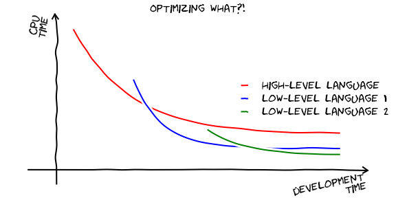
(from Johansson’s Scientific Python Lectures )
Python lies in the second category. It is easy to learn and fast to develop. It is not particularly fast but with the right tools you can increase its performance over time.
That is the reason why Python has a strong position in scientific computing. You start getting results very early during the development process. With time and effort, you can improve performance and get close to lower level programming languages.
On the other hand working with low-level languages like C or Fortran you have to write quite an amount of code to start getting the first results.
Programmer vs Scripter
You do not need to be a Python Programmer to use and take advantage of Python for your research. Have you ever found doing the same operation on a computer over and over again? simply because you do not know how to do it differently.
Scripts are not bad programs, they are simply quick and dirt, pieces of code that help you save your brain to better purposes. They are dirty because typically they are not commented, they are not actively maintained, no unitary tests, no continuous integration, no test farms, nothing of such things that first-class software usually relies on to remain functional over time.
For programs, there are those who write programs, integrated pieces of code that are intended to be used independently. Some write libraries, sets of functions, classes, routines, and methods, as you prefer to call them. Those are the building blocks of larger structures, such as programs or other libraries.
As a scientist that uses computing to pursue your research, you could be doing scripts, doing programs, or doing libraries. There is nothing pejorative in doing scripts, and there is nothing derogatory in using scripting languages. The important is the science, get the job done, and move forward.
In addition to Scripts and Programs, Python can be used in interactive computing. This document that you see right now was created as a Jupyter notebook. If you are reading it from an active Jupyter instance, you can execute these boxes.
Example 1: Program that converts from Fahrenheit to Celsius
Lets start with a simple example converting a variable that holds a value in Fahrenheit and convert it to Celsius
First code
f=80 # Temperature in F

c = 5/9 * (f-32)

print("The temperature of %.2f F is equal to %.2f C" % (f,c))
The temperature of 80.00 F is equal to 26.67 C
Second code
Now that we know how to convert from Fahrenheit to Celsius we can put the formula inside a function. Even better we want to write two functions, one to convert from F to C and the other to convert from C to F.
def fahrenheit2celsius(f):
    return 5/9 * (f-32)

def celsius2fahrenheit(c):
    return c*9/5 + 32
With this two functions we can use them to convert temperatures between these units.
fahrenheit2celsius(80)
26.666666666666668
celsius2fahrenheit(27)
80.6
We have learned here the use of variables, the print function and how to write functions in Python.
Testing your Python Environment
We will now explore a little bit about how things work in python. The purpose of this section is two-fold, to give you a quick overview of the kind of things that you can do with Python and to test if those things work for you, in particular the external libraries that could still not be present in your system. The most basic thing you can do is use the Python interpreter as a calculator, and test for example a simple operation to count the number of days on a non-leap year:
31*7 + 30*4 + 28
365
Python provides concise methods for handling lists without explicit use of loops.
They are called list comprehension, we will discuss them in more detail later on. I search for a very obfuscating case indeed!
n = 100
primes = [prime for prime in range(2, n) if prime not in
          [noprimes for i in range(2, int(n**0.5)) for noprimes in
           range(i * 2, n, i)]]
print(primes)
[2, 3, 5, 7, 11, 13, 17, 19, 23, 29, 31, 37, 41, 43, 47, 53, 59, 61, 67, 71, 73, 79, 83, 89, 97]
Python’s compact syntax: The quicksort algorithm
Python is a high-level, dynamically typed multiparadigm programming language. Python code is often said to be almost like pseudocode since it allows you to express very powerful ideas in very few lines of code while being very readable.
As an example, here is an implementation of the classic quicksort algorithm in Python:
def quicksort(arr):
    if len(arr) <= 1:
        return arr
    pivot = arr[len(arr) // 2]
    left = [x for x in arr if x < pivot]
    middle = [x for x in arr if x == pivot]
    right = [x for x in arr if x > pivot]
    return quicksort(left) + middle + quicksort(right)

print(quicksort([3,6,8,10,1,2,1]))
[1, 1, 2, 3, 6, 8, 10]
As comparison look for an equivalent version of the same algorithm implemented in C, based on a similar implementation on RosettaCode
#include
void quicksort(int *A, int len);
int main (void) { int a[] = {3,6,8,10,1,2,1}; int n = sizeof a / sizeof a[0];
int i; for (i = 0; i < n; i++) { printf(“%d “, a[i]); } printf(“\n”);
quicksort(a, n);
for (i = 0; i < n; i++) { printf(“%d “, a[i]); } printf(“\n”);
return 0; }
void quicksort(int *A, int len) { if (len < 2) return;
int pivot = A[len / 2];
int i, j; for (i = 0, j = len - 1; ; i++, j–) { while (A[i] < pivot) i++; while (A[j] > pivot) j–;
if (i >= j) break;

int temp = A[i];
A[i]     = A[j];
A[j]     = temp;   }
quicksort(A, i); quicksort(A + i, len - i); } The most important benefits of Python is how compact the notation can be and how easy it is to write code that otherwise requires not only more coding, but also compilation.
Python, however, is in general much slower than C or Fortran. There are ways to alleviate this as we will see when we start using libraries like NumPy or external code translators like Cython.
Python versions
Today, Python 3.x is the only version actively developed and maintained. Before 2020 two versions were used the older Python 2 and the newer Python 3. Python 3 introduced many backward-incompatible changes to the language, so code is written for 2.x, in general, did not work under 3.x and vice versa.
By the time of writing this notebook (July 2022), the current version of Python is 3.10.5.
Python 2.7 is no longer maintained and you should avoid using Python 2.x for any purpose that pretends to be used by you or others in the future.
You can check your Python version at the command line by running on the terminal:
$> python --version
Python 3.10.5
Another way of checking the version from inside the Jupyter notebook like this is using:
import sys
print(sys.version)
3.11.7 (main, Dec 24 2023, 07:47:18) [Clang 12.0.0 (clang-1200.0.32.29)]
To get this we import a module called sys. This is just one of the many modules in the Python Standard Library.
The Python standard library that is always distributed with Python.
This library contains built-in modules (written in C) that provide access to system functionality such as file I/O that would otherwise be inaccessible to Python programmers, as well as other modules written in Python that provide standardized solutions for many problems that occur in everyday programming.
We will use the standard library extensively but we will first focus our attention on the language itself.
Just in case you get in your hands’ code written in the old Python 2.x at the end of this notebook you can see a quick summary of a few key differences between Python 2.x and 3.x
Example 2: The Barnsley fern
The Barnsley fern is a fractal named after the British mathematician Michael Barnsley who first described it in his book “Fractals Everywhere”. He made it to resemble the black spleenwort, Asplenium adiantum-nigrum. This fractal has served as inspiration to create natural structures using iterative mathematical functions.
Barnsley’s fern uses four affine transformation’s, i.e. simple vector transformations that include a vector-matrix multiplication and a translation. The formula for one transformation is the following:
\[f_w(x,y) = \begin{bmatrix}a & b \\ c & d \end{bmatrix} \begin{bmatrix} x \\ y \end{bmatrix} + \begin{bmatrix} e \\ f \end{bmatrix}\]Barnsley uses four transformations with weights for them to reproduce the fern leaf. The transformations are shown below.
\[\begin{align} f_1(x,y) &= \begin{bmatrix} 0.00 & 0.00 \\ 0.00 & 0.16 \end{bmatrix} \begin{bmatrix} x \\ y \end{bmatrix} \\[6px] f_2(x,y) &= \begin{bmatrix} 0.85 & 0.04 \\ -0.04 & 0.85 \end{bmatrix} \begin{bmatrix} x \\ y \end{bmatrix} + \begin{bmatrix} 0.00 \\ 1.60 \end{bmatrix} \\[6px] f_3(x,y) &= \begin{bmatrix} 0.20 & -0.26 \\ 0.23 & 0.22 \end{bmatrix} \begin{bmatrix} x \\ y \end{bmatrix} + \begin{bmatrix} 0.00 \\ 1.60 \end{bmatrix} \\[6px] f_4(x,y) &= \begin{bmatrix} -0.15 & 0.28 \\ 0.26 & 0.24 \end{bmatrix} \begin{bmatrix} x \\ y \end{bmatrix} + \begin{bmatrix} 0.00 \\ 0.44 \end{bmatrix} \end{align}\]The probability factor $p$ for the four transformations can be seen in the table below:
\[\begin{align} p[f_1] &\rightarrow 0.01 \\[6px] p[f_2] &\rightarrow 0.85 \\[6px] p[f_3] &\rightarrow 0.07 \\[6px] p[f_4] &\rightarrow 0.07 \end{align}\]The first point drawn is at the origin $(x,y)=(0,0)$ and then the new points are iteratively computed by randomly applying one of the four coordinate transformations $f_1 \cdots f_4$
We will develop this program in two stages. First, we will try to use numpy. The de facto package for dealing with numerical arrays in Python. As we already know how to write functions, lets start writing four functions for the the four transformations. In this case we can define $r$ as being the vector (x,y). This will help us defining the functions in a very compact expression.
import numpy as np
import matplotlib.pyplot as plt
def f1(r):
    a=np.array([[0,0],[0,0.16]])
    return np.dot(a,r)

def f2(r):
    a=np.array([[0.85,0.04],[-0.04, 0.85]])
    return np.dot(a,r)+np.array([0.0,1.6])

def f3(r):
    a=np.array([[0.20,-0.26],[0.23,0.22]])
    return np.dot(a,r)+np.array([0.0,1.6])

def f4(r):
    a=np.array([[-0.15, 0.28],[0.26,0.24]])
    return np.dot(a,r)+np.array([0.0,0.44])
These four functions will transform points in $r$ into new positions $r’$. We can now assemble the code to assigned the transformations according to the probability factors described above.
r0=np.array([0,0])
npoints=100000

points=np.zeros((npoints,2))

fig, ax = plt.subplots()

for i in range(npoints):
    rnd=np.random.rand()
    if rnd<=0.01:
        r1=f1(r0)
    elif rnd<=0.86:
        r1=f2(r0)
    elif rnd<=0.93:
        r1=f3(r0)
    else:
        r1=f4(r0)
    points[i]=r0
    r0=r1

ax.plot(points[:,0],points[:,1],',')
ax.set_axis_off()
ax.set_aspect(0.5)
plt.show()

Python Syntax I: Variables
Let us start with something very simple and then we will focus on different useful packages
print("Hello Word")  # Here I am adding a comment on the same line
# Comments like these will not do anything
Hello Word
Variable types, names, and reserved words
var = 8                # Integer
k = 23434235234        # Long integer (all integers in Python 3 are long integers).
pi = 3.1415926         # float (there are better ways of defining PI with numpy)
z = 1.5+0.5j           # Complex
hi = "Hello world"    # String
truth = True           # Boolean

# Assignation to an operation
radius=3.0
area=pi*radius**2
Variables can have any name but you can not use reserved language names as:
| and | as | assert | break | class | continue | def |
| del | elif | else | except | False | finally | for |
| from | global | if | import | in | is | lambda |
| None | nonlocal | not | or | pass | raise | |
| return | True | try | while | with | yield |
Other rules for variable names:
-
Can not start with a number: (example
12var) -
Can not include illegal characters such as
% & + - =, etc -
Names in upper-case are considered different than those in lower-case
Variables can receive values assigned in several ways:
x=y=z=2.5
print(x,y,z)
2.5 2.5 2.5
a,b,c=1,2,3
print(a,b,c)
1 2 3
a,b=b,a+b
print(a,b)
2 3
import sys
print(sys.version)
3.11.7 (main, Dec 24 2023, 07:47:18) [Clang 12.0.0 (clang-1200.0.32.29)]
Basic data types
Numbers
Integers and floats work as you would expect from other languages:
x = 3
print(x, type(x))
3 <class 'int'>
print(x + 1)   # Addition;
print(x - 1)   # Subtraction;
print(x * 2)   # Multiplication;
print(x ** 2)  # Exponentiation;
4
2
6
9
x += 1
print(x)  # Prints "4"
x *= 2
print(x)  # Prints "8"
4
8
y = 2.5
print(type(y)) # Prints "<type 'float'>"
print(y, y + 1, y * 2, y ** 2) # Prints "2.5 3.5 5.0 6.25"
<class 'float'>
2.5 3.5 5.0 6.25
Note that unlike many languages (C for example), Python does not recognize the unary increment (x++) or decrement (x--) operators.
Python also has built-in types for long integers and complex numbers; you can find all of the details in the Official Documentation for Numeric Types.
Basic Mathematical Operations
- With Python we can do the following basic operations:
Addition (+), subtraction
(-), multiplication
(*) and división (/).
- Other less common:
Exponentiation (**),
integer division (//) o
module (%).
Precedence of Operations
- PEDMAS
- Parenthesis
- Exponents
- Division and Multiplication.
- Addition and Substraction
- From left to right.
Let’s see some examples:
print((3-1)*2)
print(3-1 *2)
print(1/2*4)
4
1
2.0
Booleans
Python implements all of the usual operators for Boolean logic, but uses English words rather than symbols (&&, ||, etc.):
t, f = True, False
print(type(t)) # Prints "<type 'bool'>"
<class 'bool'>
answer = True
answer
True
Now let’s look at the operations:
print(t and f) # Logical AND;
print(t or f)  # Logical OR;
print(not t)   # Logical NOT;
print(t != f)  # Logical XOR;
False
True
False
True
a=10
b=20
print (a==b)
print (a!=b)
False
True
a=10
b=20
print (a>b)
print (a<b)
print (a>=b)
#print (a=>b) # Error de sintaxis
print (a<=b)
False
True
False
True
Strings
hello = 'hello'   # String literals can use single quotes
world = "world"   # or double quotes; it does not matter.
print(hello, len(hello))
hello 5
hw = hello + ' ' + world  # String concatenation
print(hw)  # prints "hello world"
hello world
hw12 = '%s %s %d' % (hello, world, 12)  # sprintf style string formatting
print(hw12)  # prints "hello world 12"
hello world 12
String objects have a bunch of useful methods; for example:
s = "Monty Python"
print(s.capitalize())  # Capitalize a string; prints "Monty python"
print(s.upper())       # Convert a string to uppercase; prints "MONTY PYTHON"
print(s.lower())       # Convert a string to lowercase; prints "monty python"
print('>|'+s.rjust(40)+'|<')    # Right-justify a string, padding with spaces
print('>|'+s.center(40)+'|<')   # Center a string, padding with spaces
print(s.replace('y', '(wye)'))  # Replace all instances of one substring with another;
                                # prints "Mont(wye) P(wye)thon"

print('>|'+'      Monty Python    '.strip()+'|<')  # Strip leading and trailing whitespace
Monty python
MONTY PYTHON
monty python
>|                            Monty Python|<
>|              Monty Python              |<
Mont(wye) P(wye)thon
>|Monty Python|<
We can see a more general picture on how to slice a string as
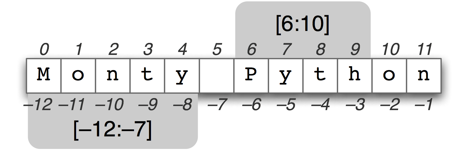
#  strings I

word = "Monty Python"
part = word[6:10]
print (part)
part = word[:4]
print(part)
part = word[5:]
print(part)
part = word[1:8:2] # from 1 to 8 in spaces of 2
print(part)
rev = word [::-1]
print(rev)
text = 'a,b,c'
text = text.split(',')
print(text)

c1="my.My.my.My"
c2="name"
c1+c2
c1*3
c1.split(".")
Pyth
Mont
 Python
ot y
nohtyP ytnoM
['a', 'b', 'c']


['my', 'My', 'my', 'My']
Today’s programs need to be able to handle a wide variety of characters. Applications are often internationalized to display messages and output in a variety of user-selectable languages; the same program might need to output an error message in English, French, Japanese, Hebrew, or Russian. Web content can be written in any of these languages and can also include a variety of emoji symbols. Python’s string type uses the Unicode Standard for representing characters, which lets Python programs work with all these different possible characters.
Unicode (https://www.unicode.org/) is a specification that aims to list every character used by human languages and give each character its unique code. The Unicode specifications are continually revised and updated to add new languages and symbols.
UTF-8 is one of the most commonly used encodings, and Python often defaults to using it.
You can find a list of all string methods in the Python 3.10 Language Documentation for Text sequence type (str).
String Formatting and text printing
In Python 3.x and higher, print() is a normal function as any other (so print(2, 3) prints “2 3”.
If you see a code with a line like:
print 2, 3
This code is using Python 2.x syntax. This is just one of the backward incompatible differences introduced in Python 3.x. In Python 2.x and before print was a statement like if or for. In Python 3.x the statement was removed in favor of a function.
print("Hellow word!")
print()
print(7*3)
Hellow word!

21
name = "Theo"
print("His names is : ", name)
print()
grade = 19.5
neval = 3
print("Average : ", grade/neval),

# array
a = [1, 2, 3, 4]

# printing a element in same
# line
for i in range(4):
    print(a[i], end =" ")
His names is :  Theo

Average :  6.5
1 2 3 4
There are four major ways to do string formatting in Python. These ways have evolved from the origin of the language itself trying to mimic the ways of other languages such as C or Fortran that have used certain formatting techniques for a long time.
Old style String Formatting (The % operator)
Strings in Python have a unique built-in operation that can be accessed with the % operator.
This lets you do simple positional formatting very easily.
This operator due its existence to the old printf-style function in C language. In C printf is a function that can receive several arguments. The string return is based on the first string and variables replaced with some special characters indicating the format of the variable should take as a string.
| %s | *string*. | |
| %d | integer. | |
| %0xd | an integer with x zeros from the left. | |
| %f | decimal notation with six digits. | |
| %e | scientific notation (compact) with e in the exponent. |
|
| %E | scientific notation (compact) with E in the exponent. |
|
| %g | decimal or scientific notation with e in the exponent. |
|
| %G | decimal or scientific notation with E in the exponent. |
|
| %xz | format z adjusted to the rigth in a field of width x. | |
| %-xz | format z adjusted to the left in a field of width x. | |
| %.yz | format z with y digits. | |
| %x.yz | format z with y digits in afield of width x . | |
| %% | percentage sign. |
See some examples of the use of this notation.
n = 15          # Int
r = 3.14159     # Float
s = "Hiii"      # String
print("|%4d, %6.4f|" % (n,r))
print("%e, %g" % (r,r))
print("|%2s, %4s, %5s, %10s|" % (s, s, s ,s))
|  15, 3.1416|
3.141590e+00, 3.14159
|Hiii, Hiii,  Hiii,       Hiii|
'Hello, %s' % name
'Hello, Theo'
'The name %s has %d characters' % (name, len(name))
'The name Theo has 4 characters'
The new style String Formatting (str.format)
Python 3 introduced a new way to do string formatting. This “new style” string formatting gets rid of the %-operator special syntax and makes the syntax for string formatting more regular. Formatting is now handled by calling .format() on a string object.
You can use format() to do simple positional formatting, just like you could with “old style” formatting:
'Hello, {}'.format(name)
'Hello, Theo'
'The name {username} has {numchar} characters'.format(username=name, numchar= len(name))
'The name Theo has 4 characters'
In Python 3.x, this “new style” string formatting is to be preferred over %-style formatting. While “old style” formatting has been de-emphasized, it has not been deprecated. It is still supported in the latest versions of Python.
The even newer String Formatting style (Since Python 3.6)
Python 3.6 added a new string formatting approach called formatted string literals or “f-strings”. This new way of formatting strings lets you use embedded Python expressions inside string constants. Here’s a simple example to give you a feel for the feature:
f'The name {name} has {len(name)} characters'
'The name Theo has 4 characters'
Here we are not printing, just creating a string with replacements done on-the-fly indicated by the presence of the f'' before the string. You can do operations inside the string for example:
a = 2
b = 3
f'The sum of {a} and {b} is {a + b}, the product is {a*b} and the power {a}^{b} = {a**b}'
'The sum of 2 and 3 is 5, the product is 6 and the power 2^3 = 8'
Template Strings (Standard Library)
Here’s one more tool for string formatting in Python: template strings. It’s a simpler and less powerful mechanism, but in some cases, this might be exactly what you’re looking for.
from string import Template

t = Template('The name $name has $numchar characters')
t.substitute(name=name, numchar=len(name))
'The name Theo has 4 characters'
Python Syntax II: Sequence and Mapping Types. loops and conditionals
Python includes several built-in container types: lists, dictionaries, sets, and tuples. They are particularly useful when you are working with loops and conditionals. We will cover all these language elements here
Lists
The items of a list are arbitrary Python objects. Lists are formed by placing a comma-separated list of expressions in square brackets. (Note that there are no special cases needed to form lists of length 0 or 1.).
Lists are mutable meaning that they can be changed after they are created.
xs = [8, 4, 2]    # Create a list
print(xs, xs[2])
print(xs[-1])     # Negative indices count from the end of the list; prints "2"
[8, 4, 2] 2
2
xs[2] = 'cube'     # Lists can contain elements of different types
print(xs)
[8, 4, 'cube']
xs.append('tetrahedron')  # Add a new element to the end of the list
print(xs)
[8, 4, 'cube', 'tetrahedron']
x = xs.pop()      # Remove and return the last element of the list
print(x, xs)
tetrahedron [8, 4, 'cube']
words = ["triangle", ["square", "rectangle", "rhombus"], "pentagon"]
print(words[1][2])
rhombus
As usual, you can find all the more details about mutable in the Python 3.10 documentation for sequence types.
Slicing
In addition to accessing list elements one at a time, Python provides concise syntax to access sublists; this is known as slicing:
nums = range(5)      # range in Python 3.x is a built-in function that creates an iterable
lnums = list(nums)
print(lnums)         # Prints "[0, 1, 2, 3, 4]"
print(lnums[2:4])    # Get a slice from index 2 to 4 (excluding 4); prints "[2, 3]"
print(lnums[2:])     # Get a slice from index 2 to the end; prints "[2, 3, 4]"
print(lnums[:2])     # Get a slice from the start to index 2 (excluding 2); prints "[0, 1]"
print(lnums[:])      # Get a slice of the whole list; prints ["0, 1, 2, 3, 4]"
print(lnums[:-1])    # Slice indices can be negative; prints ["0, 1, 2, 3]"
lnums[2:4] = [8, 9] # Assign a new sublist to a slice
print(lnums)         # Prints "[0, 1, 8, 9, 4]"
[0, 1, 2, 3, 4]
[2, 3]
[2, 3, 4]
[0, 1]
[0, 1, 2, 3, 4]
[0, 1, 2, 3]
[0, 1, 8, 9, 4]
Loops over lists
You can loop over the elements of a list like this:
platonic=['Tetrahedron', 'Cube', 'Octahedron', 'Dodecahedron', 'Icosahedron']
for solid in platonic:
    print(solid)
Tetrahedron
Cube
Octahedron
Dodecahedron
Icosahedron
If you want access to the index of each element within the body of a loop, use the built-in enumerate function:
platonic=['Tetrahedron', 'Cube', 'Octahedron', 'Dodecahedron', 'Icosahedron']
for idx, solid in enumerate(platonic):
    print('#%d: %s' % (idx + 1, solid))
#1: Tetrahedron
#2: Cube
#3: Octahedron
#4: Dodecahedron
#5: Icosahedron
Copying lists:
# Assignment statements
# Incorrect copy

L=[]
M=L

# modify both lists
L.append('a')
print(L, M)

M.append('asd')
print(L,M)
['a'] ['a']
['a', 'asd'] ['a', 'asd']
#Shallow copy

L=[]
M=L[:]         # Shallow copy using slicing
N=list(L)      # Creating another shallow copy

# modify only one
L.append('a')
print(L, M, N)
['a'] [] []
Shallow copy vs Deep Copy
Assignment statements in Python do not copy objects, they create bindings between a target and an object. Therefore, the problem with shallow copies is that internal objects are only referenced
lst1 = ['a','b',['ab','ba']]
lst2 = lst1[:]
lst2[2][0]='cd'
print(lst1)
['a', 'b', ['cd', 'ba']]
lst1 = ['a','b',['ab','ba']]
lst2 = list(lst1)
lst2[2][0]='cd'
print(lst1)
['a', 'b', ['cd', 'ba']]
To produce a deep copy you can use a module from the Python Standard Library. The Python Standard library will be covered in the next Notebook, however, this is a good place to clarify this important topic about Shallow and Deep copies in Python.
from copy import deepcopy

lst1 = ['a','b',['ab','ba']]
lst2 = deepcopy(lst1)
lst2[2][0]='cd'
print(lst1)
['a', 'b', ['ab', 'ba']]
Deleting lists:
platonic=['Tetrahedron', 'Cube', 'Octahedron', 'Dodecahedron', 'Icosahedron']
print(platonic)
del platonic

try: platonic
except NameError: print("The variable 'platonic' is not defined")
['Tetrahedron', 'Cube', 'Octahedron', 'Dodecahedron', 'Icosahedron']
The variable 'platonic' is not defined
platonic=['Tetrahedron', 'Cube', 'Octahedron', 'Dodecahedron', 'Icosahedron']
del platonic[1]
print(platonic)
del platonic[-1]                  #Delete last element
print(platonic)

platonic=['Tetrahedron', 'Cube', 'Octahedron', 'Dodecahedron', 'Icosahedron']
platonic.remove("Cube")
print(platonic)

newl=["Circle", 2]
print(platonic+newl)
print(newl*2)
print(2*newl)
['Tetrahedron', 'Octahedron', 'Dodecahedron', 'Icosahedron']
['Tetrahedron', 'Octahedron', 'Dodecahedron']
['Tetrahedron', 'Octahedron', 'Dodecahedron', 'Icosahedron']
['Tetrahedron', 'Octahedron', 'Dodecahedron', 'Icosahedron', 'Circle', 2]
['Circle', 2, 'Circle', 2]
['Circle', 2, 'Circle', 2]
Sorting lists:
list1=['Tetrahedron', 'Cube', 'Octahedron', 'Dodecahedron', 'Icosahedron']
list2=[1,200,3,10,2,999,-1]
list1.sort()
list2.sort()
print(list1)
print(list2)
['Cube', 'Dodecahedron', 'Icosahedron', 'Octahedron', 'Tetrahedron']
[-1, 1, 2, 3, 10, 200, 999]
List comprehensions:
When programming, frequently we want to transform one type of data into another. As a simple example, consider the following code that computes square numbers:
nums = [0, 1, 2, 3, 4]
squares = []
for x in nums:
    squares.append(x ** 2)
print(squares)
[0, 1, 4, 9, 16]
You can make this code simpler using a list comprehension:
nums = [0, 1, 2, 3, 4]
squares = [x ** 2 for x in nums]
print(squares)
[0, 1, 4, 9, 16]
List comprehensions can also contain conditions:
nums = [0, 1, 2, 3, 4]
even_squares = [x ** 2 for x in nums if x % 2 == 0]
print(even_squares)
[0, 4, 16]
Dictionaries
A dictionary stores (key, value) pairs, similar to a Map in Java or an object in Javascript. You can use it like this:
# Create a new dictionary with some data about regular polyhedra
rp = {'Tetrahedron': 4, 'Cube': 6, 'Octahedron': 8, 'Dodecahedron': 12, 'Icosahedron': 20}
print(rp['Cube'])              # Get an entry from a dictionary; prints "cute"
print('Icosahedron' in rp)     # Check if a dictionary has a given key; prints "True"
6
True
rp['Circle'] = 0         # Set an entry in a dictionary
print(rp['Circle'])      # Prints "0"
0
'Heptahedron' in rp
False
print(rp.get('Hexahedron', 'N/A'))  # Get an element with a default; prints "N/A"
print(rp.get('Cube', 'N/A'))        # Get an element with a default; prints 6
N/A
6
del rp['Circle']        # Remove an element from a dictionary
print(rp.get('Circle', 'N/A')) # "Circle" is no longer a key; prints "N/A"
N/A
You can find all you need to know about dictionaries in the Python 3.10 documentation for Mapping types.
It is easy to iterate over the keys in a dictionary:
rp = {'Tetrahedron': 4, 'Cube': 6, 'Octahedron': 8, 'Dodecahedron': 12, 'Icosahedron': 20}
for polyhedron in rp:
    faces = rp[polyhedron]
    print('The %s has %d faces' % (polyhedron.lower(), faces))

for n in rp.keys():
    print(n,rp[n])
The tetrahedron has 4 faces
The cube has 6 faces
The octahedron has 8 faces
The dodecahedron has 12 faces
The icosahedron has 20 faces
Tetrahedron 4
Cube 6
Octahedron 8
Dodecahedron 12
Icosahedron 20
If you want access to keys and their corresponding values, use the items() method. This is an iterable, not a list.
rp = {'Tetrahedron': 4, 'Cube': 6, 'Octahedron': 8, 'Dodecahedron': 12, 'Icosahedron': 20}
for polyhedron, faces in rp.items():
    print('The %s has %d faces' % (polyhedron, faces))
The Tetrahedron has 4 faces
The Cube has 6 faces
The Octahedron has 8 faces
The Dodecahedron has 12 faces
The Icosahedron has 20 faces
Dictionary comprehensions: These are similar to list comprehensions, but allow you to easily construct dictionaries. For example:
nums = [0, 1, 2, 3, 4]
even_num_to_square = {x: x ** 2 for x in nums if x % 2 == 0}
print(even_num_to_square)
{0: 0, 2: 4, 4: 16}
Sets
A set is an unordered collection of distinct elements. As a simple example, consider the following:
polyhedron = {'tetrahedron', 'hexahedron', 'icosahedron'}
print('tetrahedron' in polyhedron)   # Check if an element is in a set; prints "True"
print('sphere' in polyhedron)    # prints "False"
True
False
polyhedron.add('cube')        # Add an element to a set
print('cube' in polyhedron)
print(len(polyhedron))       # Number of elements in a set;
True
4
polyhedron.add('hexahedron')   # Adding an element that is already in the set does nothing
print(polyhedron)
polyhedron.remove('cube')      # Remove an element from a set
print(polyhedron)
{'hexahedron', 'cube', 'tetrahedron', 'icosahedron'}
{'hexahedron', 'tetrahedron', 'icosahedron'}
setA = set(["first", "second", "third", "first"])
print("SetA = ",setA)
setB = set(["second", "fourth"])
print("SetB=",setB)

print(setA & setB)                       # Intersection
print(setA | setB)                       # Union
print(setA - setB)                       # Difference A-B
print(setB - setA)                       # Difference B-A
print(setA ^ setB)                       # symmetric difference
set(['fourth', 'first', 'third'])

# Set is not mutable, elements of the frozen set remain the same after creation
immutable_set = frozenset(["a", "b", "a"])
print(immutable_set)
SetA =  {'third', 'first', 'second'}
SetB= {'fourth', 'second'}
{'second'}
{'third', 'first', 'second', 'fourth'}
{'third', 'first'}
{'fourth'}
{'fourth', 'third', 'first'}
frozenset({'a', 'b'})
Loops over sets
Iterating over a set has the same syntax as iterating over a list; however since sets are unordered, you cannot make assumptions about the order in which you visit the elements of the set:
animals = {'cat', 'dog', 'fish'}
for idx, animal in enumerate(animals):
    print('#%d: %s' % (idx + 1, animal))
# Prints "#1: fish", "#2: dog", "#3: cat"
#1: dog
#2: cat
#3: fish
Set comprehensions: Like lists and dictionaries, we can easily construct sets using set comprehensions:
from math import sqrt
lc=[int(sqrt(x)) for x in range(30)]
sc={int(sqrt(x)) for x in range(30)}

print(lc)
print(sc)
[0, 1, 1, 1, 2, 2, 2, 2, 2, 3, 3, 3, 3, 3, 3, 3, 4, 4, 4, 4, 4, 4, 4, 4, 4, 5, 5, 5, 5, 5]
{0, 1, 2, 3, 4, 5}
set(lc)
{0, 1, 2, 3, 4, 5}
Tuples
A tuple is an (immutable) ordered list of values. A tuple is in many ways similar to a list; one of the most important differences is that tuples can be used as keys in dictionaries and as elements of sets, while lists cannot.
Some general observations on tuples are:
1) A tuple can not be modified after its creation.
2) A tuple is defined similarly to a list, only that the set is enclosed with parenthesis, “()”, instead of “[]”.
3) The elements in the tuple have a predefined order, similar to a list.
4) Tuples have the first index as zero, similar to lists, such that t[0] always exist.
5) Negative indices count from the end, as in lists.
6) Slicing works as in lists.
7) Extracting sections of a list gives a list, similarly, a section of a tuple, gives a tuple.
8) append or sort do not work in tuples. “in” can be used to know if an element exists in a tuple.
9) Tuples are much faster than lists.
10) If you are defining a fixed set of values and the only thing you would do is to run over it, use a tuple instead of a list.
11) Tuples can be converted in lists list(tuple) and lists in tuples tuple(list)
d = {(x, x + 1): x for x in range(10)}  # Create a dictionary with tuple keys
t = (5, 6)       # Create a tuple
print(type(t))
print(d[t])
print(d[(1, 2)])
print(d)
e = (1,2,'a','b')
print(type(e))
#print('MIN of Tuple=',min(e))

e = (1,2,3,4)
print('MIN of Tuple=',min(e))

word = 'abc'
L = list(word)
lp=list(word)
tp=tuple(word)
print(lp,tp)
<class 'tuple'>
5
1
{(0, 1): 0, (1, 2): 1, (2, 3): 2, (3, 4): 3, (4, 5): 4, (5, 6): 5, (6, 7): 6, (7, 8): 7, (8, 9): 8, (9, 10): 9}
<class 'tuple'>
MIN of Tuple= 1
['a', 'b', 'c'] ('a', 'b', 'c')
#TypeError: 'tuple' object does not support item assignment

#t[0] = 1
Conditionals
-
Conditionals are expressions that can be true or false. For example
- have the user type the correct word?
- is the number bigger than 100?
-
The result of the conditions will decide what will happen, for example:
- When the input word is correct, print “Good”
- To all numbers larger than 100 subtract 20.
Boolean Operators
x = 125
y = 251

print(x == y)    # x equal to y
print(x != y)    # x is not equal to y
print(x >  y)    # x is larger than y
print(x <  y)    # x is smaller than y
print(x >= y)    # x is larger or equal than y
print(x <= y)    # x is smaller or equal than y
print(x == 125)  # x is equal to 125
False
True
False
True
False
True
True
passwd = "nix"
num  = 10
num1 = 20
letter = "a"

print(passwd == "nix")
print(num >= 0)
print(letter > "L")
print(num/2 == (num1-num))
print(num %5 != 0)
True
True
True
False
False
s1="A"
s2="Z"

print(s1>s2)
print(s1.isupper())
print(s1.lower()>s2)
False
True
True
Conditional (if…elif…else)
# Example with the instruction if
platonic = {4: "tetrahedron",
            6: "hexahedron",
            8: "octahedron",
            12: "dodecahedron",
            20: "icosahedron"}

num_faces = 6

if num_faces in platonic.keys():
    print(f"There is a regular solid with {num_faces} faces and the name is {platonic[num_faces]}")
else:
    print(f"Theres is no regular polyhedron with {num_faces} faces")

#The of the compact form of  if...else

evenless = "Polyhedron exists" if (num_faces in platonic.keys()) else "Polyhedron does not exist"
print(evenless)
There is a regular solid with 6 faces and the name is hexahedron
Polyhedron exists
# Example of if...elif...else
x=-10

if x<0 :
    print(x," is negative")
elif x==0 :
    print("the number is zero")
else:
    print(x," is positive")
-10 is negative
# example of the keyword pass

if x<0:
   print("x is negative")
else:
   pass # I will not do anything
x is negative
Loop with conditional (while)
# Example with while

x=0
while x < 10:
     print(x)
     x = x+1
print("End")
0
1
2
3
4
5
6
7
8
9
End
# A printed table with tabular with while

x=1

while x < 10:
     print(x, "\t", x*x)
     x = x+1
1 	 1
2 	 4
3 	 9
4 	 16
5 	 25
6 	 36
7 	 49
8 	 64
9 	 81
# Comparing while and for in a string
word = "program of nothing"
index=0
while index < len(word):
    print(word[index], end ="")
    index +=1
print()
for letter in word:
      print(letter,end="")
program of nothing
program of nothing
#Using enumerate for lists

colors=["red", "green", "blue"]
for c in colors:
    print(c,end=" ")
print()
for i, col in enumerate(colors):
    print(i,col)
red green blue
0 red
1 green
2 blue
#Running over several lists at the same time

colors1 =["rojo","verde", "azul"]
colors2 =["red", "green", "blue"]
for ce, ci in zip(colors1,colors2):
    print("Color",ce,"in Spanish means",ci,"in english")
Color rojo in Spanish means red in english
Color verde in Spanish means green in english
Color azul in Spanish means blue in english
List of numbers (range)
print(list(range(10)))
print(list(range(2,10)))
print(list(range(0,11,2)))
[0, 1, 2, 3, 4, 5, 6, 7, 8, 9]
[2, 3, 4, 5, 6, 7, 8, 9]
[0, 2, 4, 6, 8, 10]
A simple application of the function range() is when we try to calculate
finite sums of integers. For example
\begin{equation} \boxed{ \sum_{i=1}^n i = \frac{n(n+1)}2\ , \ \ \ \ \ \sum_{i=1}^n i^2 = \frac{n(n+1)(2n+1)}6\ . } \end{equation}
n = 100

sum_i=0
sum_ii=0
for i in range(1,n+1):
     sum_i = sum_i + i
     sum_ii += i*i
print(sum_i, n*(n+1)/2)
print(sum_ii, n*(n+1)*(2*n+1)/6)
5050 5050.0
338350 338350.0
Loop modifiers: break and continue
for n in range(1,10):
      c=n*n
      if c > 50:
            print(n, "to the square is ",c," > 50")
            print("STOP")
            break
      else:
            print(n," with square ",c)

for i in range(-5,5,1):
    if i == 0:
        continue
    else:
        print(round(1/i,3))
1  with square  1
2  with square  4
3  with square  9
4  with square  16
5  with square  25
6  with square  36
7  with square  49
8 to the square is  64  > 50
STOP
-0.2
-0.25
-0.333
-0.5
-1.0
1.0
0.5
0.333
0.25
Python Syntax III: Functions
A function defines a set of instructions or a piece of a code with an associated name that performs a specific task and it can be re-utilized.
It can have an argument(s) or not, it can return values or not.
The functions can be given by the language, imported from an external file (module), or created by you
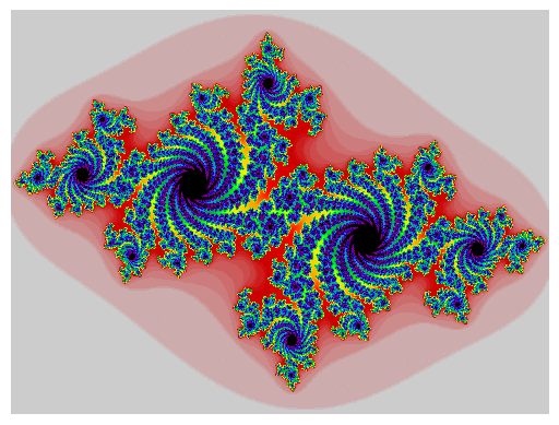
Example 3: Julia Sets
"""
Solution from:
https://codereview.stackexchange.com/questions/210271/generating-julia-set
"""
from functools import partial
from numbers import Complex
from typing import Callable

import matplotlib.pyplot as plt
import numpy as np


def douady_hubbard_polynomial(z: Complex,
                              c: Complex) -> Complex:
    """
    Monic and centered quadratic complex polynomial
    https://en.wikipedia.org/wiki/Complex_quadratic_polynomial#Map
    """
    return z ** 2 + c


def julia_set(mapping: Callable[[Complex], Complex],
              *,
              min_coordinate: Complex,
              max_coordinate: Complex,
              width: int,
              height: int,
              iterations_count: int = 256,
              threshold: float = 2.) -> np.ndarray:
    """
    As described in https://en.wikipedia.org/wiki/Julia_set
    :param mapping: function defining Julia set
    :param min_coordinate: bottom-left complex plane coordinate
    :param max_coordinate: upper-right complex plane coordinate
    :param height: pixels in vertical axis
    :param width: pixels in horizontal axis
    :param iterations_count: number of iterations
    :param threshold: if the magnitude of z becomes greater
    than the threshold we assume that it will diverge to infinity
    :return: 2D pixels array of intensities
    """
    im, re = np.ogrid[min_coordinate.imag: max_coordinate.imag: height * 1j,
                      min_coordinate.real: max_coordinate.real: width * 1j]
    z = (re + 1j * im).flatten()

    live, = np.indices(z.shape)  # indexes of pixels that have not escaped
    iterations = np.empty_like(z, dtype=int)

    for i in range(iterations_count):
        z_live = z[live] = mapping(z[live])
        escaped = abs(z_live) > threshold
        iterations[live[escaped]] = i
        live = live[~escaped]
        if live.size == 0:
            break
    else:
        iterations[live] = iterations_count

    return iterations.reshape((height, width))
mapping = partial(douady_hubbard_polynomial,
                  c=-0.7 + 0.27015j)  # type: Callable[[Complex], Complex]

image = julia_set(mapping,
                  min_coordinate=-1.5 - 1j,
                  max_coordinate=1.5 + 1j,
                  width=800,
                  height=600)
plt.axis('off')
plt.imshow(image,
           cmap='nipy_spectral_r',
           origin='lower')
plt.savefig("julia_python.png")
plt.show()
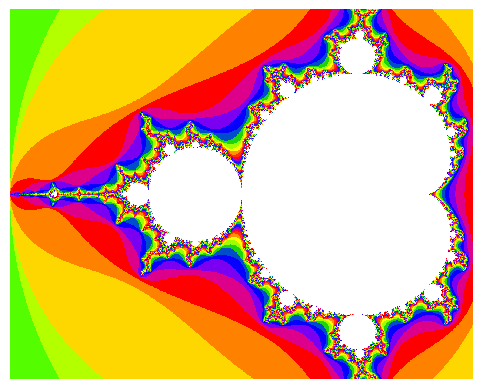
Example 4: Mandelbrot Set
import matplotlib.pyplot as plt
from pylab import arange, zeros, xlabel, ylabel
from numpy import NaN

def m(a):
    z = 0
    for n in range(1, 100):
        z = z**2 + a
        if abs(z) > 2:
            return n
    return NaN

X = arange(-2, .5, .002)
Y = arange(-1,  1, .002)
Z = zeros((len(Y), len(X)))

for iy, y in enumerate(Y):
    #print (iy, "of", len(Y))
    for ix, x in enumerate(X):
        Z[iy,ix] = m(x + 1j * y)

plt.imshow(Z, cmap = plt.cm.prism_r, interpolation = 'none', extent = (X.min(), X.max(), Y.min(), Y.max()))
xlabel("Re(c)")
ylabel("Im(c)")
plt.axis('off')
plt.savefig("mandelbrot_python.png")
plt.show()
Some Built-in functions
To see which functions are available in python, go to the web site Python 3.10 Documentation for Built-in Functions
float(obj): convert a string or a number (integer or long integer) into a float number.
int(obj): convert a string or a number (integer or long integer) into an integer.
str(num): convert a number into a string.
divmod(x,y): return the results from x/y y x%y.
pow(x,y): return x to the power y.
range(start,stop,step): return a list of number from start to stop-1 in steps.
round(x,n): return a float value x rounding to n digits after the decimal point. If n is omitted, the value per default is zero.
len(obj): return the len of string, lista, tupla o diccionary.
Modules from Python Standard Library
We will see more about these functions on the next notebook We will show here just a few from the math module
import math
math.sqrt(2)
1.4142135623730951
math.log10(10000)
4.0
math.hypot(3,4)
5.0
Back in the 90’s many scientific handheld calculators could not compute factorials beyond $69!$. Let’s see in Python:
math.factorial(70)
11978571669969891796072783721689098736458938142546425857555362864628009582789845319680000000000000000
float(math.factorial(70))
1.1978571669969892e+100
import calendar

calendar.prcal(2024)
calendar.prmonth(2024, 7)
                                  2024

      January                   February                   March
Mo Tu We Th Fr Sa Su      Mo Tu We Th Fr Sa Su      Mo Tu We Th Fr Sa Su
 1  2  3  4  5  6  7                1  2  3  4                   1  2  3
 8  9 10 11 12 13 14       5  6  7  8  9 10 11       4  5  6  7  8  9 10
15 16 17 18 19 20 21      12 13 14 15 16 17 18      11 12 13 14 15 16 17
22 23 24 25 26 27 28      19 20 21 22 23 24 25      18 19 20 21 22 23 24
29 30 31                  26 27 28 29               25 26 27 28 29 30 31

       April                      May                       June
Mo Tu We Th Fr Sa Su      Mo Tu We Th Fr Sa Su      Mo Tu We Th Fr Sa Su
 1  2  3  4  5  6  7             1  2  3  4  5                      1  2
 8  9 10 11 12 13 14       6  7  8  9 10 11 12       3  4  5  6  7  8  9
15 16 17 18 19 20 21      13 14 15 16 17 18 19      10 11 12 13 14 15 16
22 23 24 25 26 27 28      20 21 22 23 24 25 26      17 18 19 20 21 22 23
29 30                     27 28 29 30 31            24 25 26 27 28 29 30

        July                     August                  September
Mo Tu We Th Fr Sa Su      Mo Tu We Th Fr Sa Su      Mo Tu We Th Fr Sa Su
 1  2  3  4  5  6  7                1  2  3  4                         1
 8  9 10 11 12 13 14       5  6  7  8  9 10 11       2  3  4  5  6  7  8
15 16 17 18 19 20 21      12 13 14 15 16 17 18       9 10 11 12 13 14 15
22 23 24 25 26 27 28      19 20 21 22 23 24 25      16 17 18 19 20 21 22
29 30 31                  26 27 28 29 30 31         23 24 25 26 27 28 29
                                                    30

      October                   November                  December
Mo Tu We Th Fr Sa Su      Mo Tu We Th Fr Sa Su      Mo Tu We Th Fr Sa Su
    1  2  3  4  5  6                   1  2  3                         1
 7  8  9 10 11 12 13       4  5  6  7  8  9 10       2  3  4  5  6  7  8
14 15 16 17 18 19 20      11 12 13 14 15 16 17       9 10 11 12 13 14 15
21 22 23 24 25 26 27      18 19 20 21 22 23 24      16 17 18 19 20 21 22
28 29 30 31               25 26 27 28 29 30         23 24 25 26 27 28 29
                                                    30 31
     July 2024
Mo Tu We Th Fr Sa Su
 1  2  3  4  5  6  7
 8  9 10 11 12 13 14
15 16 17 18 19 20 21
22 23 24 25 26 27 28
29 30 31
Functions from external modules
These functions come from modules. The way to do so is by doing
import module_name
Once it is imported, we can use the functions contained in this module by using
module_name.existing_funtion(expected_input_variables)
some module names can be long or complicated. you can then use
import module_name as mn
and then to use it, you say
mn.existing_funtion(expected_input_variables)
if you want to import only a few functions from the module, you can say
from stuff import f, g
print f("a"), g(1,2)
You can also import all function as
from stuff import *
print f("a"), g(1,2)
Combining with the nickname for the module, we can say
from stuff import f as F
from stuff import g as G
print F("a"), G(1,2)
import math

def myroot(num):
    if num<0:
         print("Enter a positive number")
         return
    print(math.sqrt(num))

# main
myroot(9)
myroot(-8)
myroot(2)
3.0
Enter a positive number
1.4142135623730951
def addthem(x,y):
   return x+y

# main
add = addthem(5,6) # Calling the function
print(add)
11
We can declare functions with optional parameters. NOTE: The optional parameters NEED to be always at the end
def operations(x,y,z=None):
    if (z==None):
        sum = x+y
        rest = x-y
        prod= x*y
        div = x/y
    else:
        sum = z+x+y
        rest = x-y-z
        prod= x*y*z
        div = x/y/z
    return sum,rest,prod,div

# main
print(operations(5,6))
a,b,c,d = operations(8,4)
print(a,b,c,d)
a,b,c,d = operations(8,4,5)
print(a,b,c,d)
(11, -1, 30, 0.8333333333333334)
12 4 32 2.0
17 -1 160 0.4
We can even pass a function to a variable and we can pass this to other function (this is called functional programming)
def operations(x,y,z=None,flag=False):
    if (flag == True):
        print("Flag is true")
    if (z==None):
        sum = x+y
        rest = x-y
        prod= x*y
        div = x/y
    else:
        sum = z+x+y
        rest = x-y-z
        prod= x*y*z
        div = x/y/z
    return sum,rest,prod,div
print(operations(5,6,flag=True))
Flag is true
(11, -1, 30, 0.8333333333333334)
Example 5: Fibonacci Sequences and Golden Ratio
At this point, you have seen enough material to start doing some initial scientific computing. Let’s start applying all that you have learned up to now.
For this introduction to Python language, we will use the Fibonacci Sequence as an excuse to start using the basics of the language.
The Fibonacci sequence is a series of numbers generated iteratively like this
$F_n=F_{n-1}+F_{n-2}$
where we can start with seeds $F_0=0$ and $F_1=1$
Starting with those seeds we can compute $F_2$, $F_3$ and so on until an arbitrary large $F_n$
The Fibonacci Sequence looks like this:
\[0,\; 1,\;1,\;2,\;3,\;5,\;8,\;13,\;21,\;34,\;55,\;89,\;144,\; \ldots\;\]Let’s play with this in our first Python program.
Let’s start by defining the first two elements in the Fibonacci series
a = 0
b = 1
We now know that we can get a new variable to store the sum of a and b
c = a + b
Remember that the built-in function range() generates the immutable sequence of numbers starting from the given start integer to the stop integer.
range(10)
range(0, 10)
The range() function doesn’t generate all numbers at once. It produces numbers one by one as the loop moves to the next number. So it consumes less memory and resources. You can get the list consuming all the values from the sequence.
list(range(10))
[0, 1, 2, 3, 4, 5, 6, 7, 8, 9]
Now we can introduce a for using the iterable range(10) loop to see the first 10 elements in the Fibonacci sequence
a = 0
b = 1
print(a)
print(b)
for i in range(10):
    c = a+b
    print(c)
    a = b
    b = c
0
1
1
2
3
5
8
13
21
34
55
89
This is a simple way to iteratively generate the Fibonacci sequence. Now, imagine that we want to store the values of the sequence.
Lists are the best containers so far, there are better options with Numpy something that we will see later.
We can just use the append method for the list and continuously add new numbers to the list.
fib = [0, 1]
for i in range(1,11):
    fib.append(fib[i]+fib[i-1])
print(fib)
[0, 1, 1, 2, 3, 5, 8, 13, 21, 34, 55, 89]
The append method works by adding the element at the end of the list.
Let’s continue with the creation of a Fibonacci function. We can create a Fibonacci function to return the Fibonacci number for an arbitrary iteration, see for example:
def fibonacci_recursive(n):
    if n < 2:
        return n
    else:
        return fibonacci_recursive(n-2) + fibonacci_recursive(n-1)
fibonacci_recursive(6)
8
We can recreate the list using this function, see the next code:
print([ fibonacci_recursive(n) for n in range (20) ])
[0, 1, 1, 2, 3, 5, 8, 13, 21, 34, 55, 89, 144, 233, 377, 610, 987, 1597, 2584, 4181]
We are using a list comprehension. There is another way to obtain the same result using the so-called lambda functions:
print(list(map(lambda x: fibonacci_recursive(x), range(20))))
[0, 1, 1, 2, 3, 5, 8, 13, 21, 34, 55, 89, 144, 233, 377, 610, 987, 1597, 2584, 4181]
lambda functions are some sort of anonymous functions. They are indeed very popular in functional programming and Python with its multiparadigm style makes lambda functions commonplace in many situations.
Using fibonacci_recursive is very inefficient of generate the Fibonacci sequence even more as n increases. The larger the value of n more calls to fibonacci_recursive is necessary.
There is an elegant solution to use the redundant recursion:
def fibonacci_fastrec(n):
    def fib(prvprv, prv, c):
        if c < 1: return prvprv
        else: return fib(prv, prvprv + prv, c - 1)
    return fib(0, 1, n)
print([ fibonacci_fastrec(n) for n in range (20) ])
[0, 1, 1, 2, 3, 5, 8, 13, 21, 34, 55, 89, 144, 233, 377, 610, 987, 1597, 2584, 4181]
This solution is still recursive but avoids the two-fold recursion from the first function.
With IPython we can use the magic %timeit to benchmark the difference between both implementations
%timeit [fibonacci_fastrec(n) for n in range (20)]
25.6 µs ± 625 ns per loop (mean ± std. dev. of 7 runs, 10,000 loops each)
%timeit [fibonacci_recursive(n) for n in range (20)]
2.18 ms ± 40.8 µs per loop (mean ± std. dev. of 7 runs, 100 loops each)
%timeit is not a Python command. It is a magic command of IPython, however, Python itself provides a more restrictive functionality. This can be provided with the time package:
import time

start = time.time()
print("hello")
end = time.time()
print(end - start)
hello
0.00046062469482421875
Finally, there is also an analytical expression for the Fibonacci sequence, so the entire recursion could be avoided.
from math import sqrt

def analytic_fibonacci(n):
    if n == 0:
        return 0
    else:
        sqrt_5 = sqrt(5);
        p = (1 + sqrt_5) / 2;
        q = 1/p;
        return int( (p**n + q**n) / sqrt_5 + 0.5 )
print([ analytic_fibonacci(n) for n in range (40) ])
[0, 1, 1, 2, 3, 5, 8, 13, 21, 34, 55, 89, 144, 233, 377, 610, 987, 1597, 2584, 4181, 6765, 10946, 17711, 28657, 46368, 75025, 121393, 196418, 317811, 514229, 832040, 1346269, 2178309, 3524578, 5702887, 9227465, 14930352, 24157817, 39088169, 63245986]
%timeit [analytic_fibonacci(n) for n in range (40)]
20.8 µs ± 3.15 µs per loop (mean ± std. dev. of 7 runs, 100,000 loops each)
There is an interesting property of the Fibonacci sequence, the ratio between consecutive elements converges to a finite value, the so-called golden number. Let us store this ratio number in a list as the Fibonacci series grow. Here we introduce the function zip() from Python. zip() is used to map the similar index of multiple containers so that they can be used just using as a single entity. As zip is not easy to understand and before we describe the Fibonacci method, let me give you a simple example of using zip
# initializing lists
sentence = [ "I", "am", "the Fibonacci", "Series" ]
first_serie = [ 1, 1, 2, 3 ]
second_serie = [ 144, 233, 377, 610 ]

mapped = zip(sentence, first_serie,second_serie)

# converting values to print as set
mapped = set(mapped)

print ("The zipped result is : ",end="")
print (mapped)

# Unzipping means converting the zipped values back to the individual self as they were.
# This is done with the help of “*” operator.

s1, s2, s3 = zip(*mapped)

print ("First string : ",end="")
print (s1)

print ("Second string : ",end="")
print (s2)

print ("Third string : ",end="")
print (s3)
The zipped result is : {('the Fibonacci', 2, 377), ('I', 1, 144), ('Series', 3, 610), ('am', 1, 233)}
First string : ('the Fibonacci', 'I', 'Series', 'am')
Second string : (2, 1, 3, 1)
Third string : (377, 144, 610, 233)
Now let us go back to Fibonacci
fib= [fibonacci_fastrec(n) for n in range (40)]
X=[ x/y for x,y in zip(fib[2:],fib[1:-1]) ]
X
[1.0,
 2.0,
 1.5,
 1.6666666666666667,
 1.6,
 1.625,
 1.6153846153846154,
 1.619047619047619,
 1.6176470588235294,
 1.6181818181818182,
 1.6179775280898876,
 1.6180555555555556,
 1.6180257510729614,
 1.6180371352785146,
 1.618032786885246,
 1.618034447821682,
 1.6180338134001253,
 1.618034055727554,
 1.6180339631667064,
 1.6180339985218033,
 1.618033985017358,
 1.6180339901755971,
 1.618033988205325,
 1.618033988957902,
 1.6180339886704431,
 1.6180339887802426,
 1.618033988738303,
 1.6180339887543225,
 1.6180339887482036,
 1.6180339887505408,
 1.6180339887496482,
 1.618033988749989,
 1.618033988749859,
 1.6180339887499087,
 1.6180339887498896,
 1.618033988749897,
 1.618033988749894,
 1.6180339887498951]
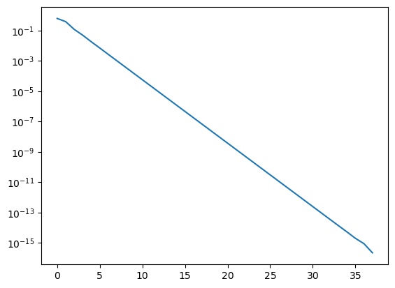
The asymptotic value of the ratio is called the Golden Ratio, its value is $\varphi = \frac{1+\sqrt{5}}{2} = 1.6180339887\ldots.$
import math

golden=(1+math.sqrt(5))/2
We can now plot how each ratio in the Fibonacci sequence is closer and closer to the golden ratio
import matplotlib.pyplot as plt

plt.semilogy([math.fabs(x - golden) for x in X]);
Functional Programming
Before we discuss object-oriented programming, it will be useful to discuss functional programming. This is the ability in python that a function can be called by another function.
The benefit of functional programming is to make your program less error-prone. Functional programming is more predictable and easier to see the outcome. Many scientific libraries adopt a functional programming paradigm.
There are several existing cases in python.
#map() function
import numpy as np

a=np.random.rand(20)
b=np.random.rand(20)

#here min is an existing function that compares two arguments, we can even create a function and use it in map
lower=map(min,a,b)
# this is an example of lazy evaluation, this is now an object, we will see the result only when we ask for the
# result.
print(lower)
#now let us see what is inside
print(list(lower))
<map object at 0x1387e9450>
[0.3479198420638585, 0.5885103951618519, 0.09788507744404285, 0.3973200826407489, 0.07151476024779557, 0.19961585086696665, 0.018736801582169504, 0.47433177615457234, 0.09502722987767931, 0.7955147481783459, 0.2968562440518463, 0.25457189637169564, 0.2402732992180341, 0.19322876498279506, 0.15700028427906199, 0.2786921343509716, 0.2323972417087179, 0.8323196759092788, 0.14846718946296644, 0.7057084437708713]
#lambda this is a method to define a function in a single line
#in this example we define a function that received three parameters and sums them up.
myfunction=lambda a,b,c: a+b+c
print(myfunction(1,2,3))

#another example
a=["phone:333333","email:al@gmail.com"]
for a in a:
    print((lambda x: x.split(":")[0] + ' ' + x.split(":")[-1])(a))
6
phone 333333
email al@gmail.com
Python Syntax IV: Object-Oriented Programming
Object-oriented programming (OOP) is a programming paradigm based on the concept of objects, which can contain data, in the form of fields (often known as attributes or properties), and code, in the form of procedures (often known as methods). A feature of objects is an object’s procedure that can access and often modify the data fields of the object with which they are associated (objects have a notion of “this” or “ self”). In OOP, computer programs are designed by making them out of objects that interact with one another.
Object-oriented programming is more than just classes and objects; it’s a whole programming paradigm based around [sic] objects (data structures) that contain data fields and methods. It is essential to understand this; using classes to organize a bunch of unrelated methods together is not object orientation.
Junade Ali, Mastering PHP Design Patterns
Class is a central concept in OOP. Classes provide means of bundling data and functionality together. Instances of a class are called objects. Each class instance can have attributes attached to it for maintaining its state. Class instances can also have methods (defined by their class) for modifying their state.
The syntax for defining classes in Python is shown with some plain examples. Anything indented in the class is within the scope of the class. Usually, they are named such that the first letter is capitalized. Variables can be defined within the class but you can also initialize some variables by calling, init, which sets the values for any parameters that need to be defined when an object is first created. You define the methods within the class but to have access to that method, you need to include self in the method signature. Now, to use, you just call the class, which then will create all variables within the class. If the class is created with some parameter, it will pass directly the variable that has been instantiated in init.
class Greeter:
    myvariable='nothing of use'


    # Constructor
    def __init__(self, name):
        self.name = name  # Create an instance variable

    # Instance method
    def greet(self, loud=False):
        if loud:
            print('HELLO, %s!' % self.name.upper())
        else:
            print('Hello, %s' % self.name)

g = Greeter('Fred')  # Construct an instance of the Greeter class
g.greet()            # Call an instance method; prints "Hello, Fred"
g.greet(loud=True)   # Call an instance method; prints "HELLO, FRED!"
Hello, Fred
HELLO, FRED!
# Let us start with a very simple class

class MyClass:
#create objects with instances customized to a specific initial state, here data is defined as an empty vector
#The self parameter is a reference to the current instance of the class,
#and is used to access variables that belong to the class
    def __init__(self):
        self.data = []
    """A simple example class"""
    i = 12345

    def f(self):
        return 'hello world'
#instantiation the class
x=MyClass
print(x.i)
print(x.f)
12345
<function MyClass.f at 0x1388a5d00>
class Person:
  def __init__(self, name, age):
    self.name = name
    self.age = age

  def myfunc(self):
    print("Hello my name is " + self.name)

p1 = Person("John", 36)


print(p1.name)
print(p1.age)
p1.myfunc()
John
36
Hello my name is John
class Rocket():
    # Rocket simulates a rocket ship for a game,
    #  or a physics simulation.

    def __init__(self):
        # Each rocket has an (x,y) position.
        self.x = 0
        self.y = 0

    def move_up(self):
        # Increment the y-position of the rocket.
        self.y += 1

# Create a fleet of 5 rockets and store them in a list.
my_rockets = [Rocket() for x in range(0,5)]

# Move the first rocket up.
my_rockets[0].move_up()

# Show that only the first rocket has moved.
for rocket in my_rockets:
    print("Rocket altitude:", rocket.y)
Rocket altitude: 1
Rocket altitude: 0
Rocket altitude: 0
Rocket altitude: 0
Rocket altitude: 0
Example 6: Quaternions
We are used to working with several numeric systems, for example:
 Natural numbers: $$\mathbb{N} \rightarrow 0, 1, 2, 3, 4, \cdots \; \text{or}\;  1, 2, 3, 4, \cdots$$

Integer numbers: $$\mathbb{Z} \rightarrow \cdots, −5, −4, −3, −2, −1, 0, 1, 2, 3, 4, 5, \cdots$$

Rational numbers: $$\mathbb{Q} \rightarrow \frac{a}{b} \;\mathrm{where}\;  a \text{and}\; b  \in \mathbb{Z} \; \mathrm{and}\; b \neq 0$$

Real numbers: $$\mathbb{R} \rightarrow \text{The limit of a convergent sequence of rational numbers. examples:}\;  \pi=3.1415..., \phi=1.61803..., etc$$

Complex numbers: $$\mathbb{C} \rightarrow a + b i \;\text{or}\; a +  i b \;\text{where}\; a \;\text{and}\; b \in \mathbb{R} \;\text{and}\; i=\sqrt{−1}$$
There are, however other sets of numbers, some of them are called hypercomplex numbers. They include the Quaternions $\mathbb{H}$, invented by Sir William Rowan Hamilton, in which multiplication is not commutative, and the Octonions $\mathbb{O}$, in which multiplication is not associative.
The use of these types of numbers is quite broad but maybe the most important use comes from engineering and computer description of moving objects, as they can be used to represent transformations of orientations of graphical objects. They are also used in Quantum Mechanics in the case of Spinors.
We will use the Quaternions as an excuse to introduce key concepts in object-oriented programming using Python. Complex numbers can be thought of as tuples of real numbers. Every complex is a real linear combination of the unit complex:
\[\lbrace e_0, e_1, \rbrace\]There are rules about how to multiply complex numbers. They can be expressed in the following table:
| $\times$ | $1$ | $i$ |
|---|---|---|
| $1$ | $1$ | $i$ |
| $i$ | $i$ | $-1$ |
Similarly, Quaternions can be thought of as 4-tuples of real numbers. Each Quaternion is a real linear combination of the unit quaternion set:
\[\lbrace e_0, e_1, e_2, e_3 \rbrace\]The rules about how to multiply Quaternions are different from Complex and Reals. They can be expressed in the following table:
| $\times$ | $1$ | $i$ | $j$ | $k$ |
|---|---|---|---|---|
| $1$ | $1$ | $i$ | $j$ |
$k$ |
| $i$ | $i$ | $-1$ | $k$ | $-j$ |
| $j$ | $j$ | $-k$ | $-1$ | $i$ |
| $k$ | $k$ | $j$ | $-i$ | $-1$ |
Our objective is to create a Python Class that could deal with Quaternions as simple and direct as possible. A class is a concept from Object-Oriented programming that allows to abstract the idea of an object. An object is something that has properties and can do things. In our case, we will create a class Quaternion. Instances of the class will be specific quaternions. We can do things with quaternions such as add two quaternions and multiply them using the multiplication rule above, we can do pretty much the same kind of things that we can expect from complex numbers but in a rather more elaborated way. Let us create a first our first version of the class Quaternion and we will improve it later on.
from numbers import Number
from math import sqrt

class Quaternion():

    def __init__(self,value=None):
        if value is None:
            self.values = tuple((0,0,0,0))
        elif isinstance(value,(int,float)):
            self.values = tuple((value, 0, 0, 0))
        elif isinstance(value,complex):
            self.values = tuple((value.real, value.imag, 0, 0))
        elif isinstance(value,(tuple, list)):
            self.values = tuple(value)

    def __eq__(self,other):
        if isinstance(other, Number):
            other= self.__class__(other)
        return self.values == other.values

    __req__ = __eq__


    def __str__(self):
        sigii = '+' if self.values[1] >= 0 else '-'
        sigjj = '+' if self.values[2] >= 0 else '-'
        sigkk = '+' if self.values[3] >= 0 else '-'
        return "%.3f %s %.3f i %s %.3f j %s %.3f k" % ( self.values[0], sigii, abs(self.values[1]), sigjj, abs(self.values[2]), sigkk, abs(self.values[3]))

    def __repr__(self):
        return 'Quaternion('+str(self.values)+')'

    @property
    def scalar_part(self):
        return self.values[0]

    @property
    def vector_part(self):
        return self.values[1:]

    @staticmethod
    def one():
        return Quaternion((1,0,0,0))

    @staticmethod
    def ii():
        return Quaternion((0,1,0,0))

    @staticmethod
    def jj():
        return Quaternion((0,0,1,0))

    @staticmethod
    def kk():
        return Quaternion((0,0,0,1))

    def __add__(self, other):
        if isinstance(other, Number):
            other = self.__class__(other)
        ret=[0,0,0,0]
        for i in range(4):
            ret[i]=self.values[i]+other.values[i]
        return self.__class__(ret)

    __radd__ = __add__


    def __mul__(self, other):
        if isinstance(other, Number):
            other = self.__class__(other)
        ret = [0,0,0,0]
        ret[0] = self.values[0]*other.values[0]-self.values[1]*other.values[1]-self.values[2]*other.values[2]-self.values[3]*other.values[3]
        ret[1] = self.values[0]*other.values[1]+self.values[1]*other.values[0]+self.values[2]*other.values[3]-self.values[3]*other.values[2]
        ret[2] = self.values[0]*other.values[2]+self.values[2]*other.values[0]+self.values[3]*other.values[1]-self.values[1]*other.values[3]
        ret[3] = self.values[0]*other.values[3]+self.values[3]*other.values[0]+self.values[1]*other.values[2]-self.values[2]*other.values[1]
        return self.__class__(ret)

    def __rmul__(self, other):
        if isinstance(other, Number):
            other= self.__class__(other)
        ret = [0,0,0,0]
        ret[0] = self.values[0]*other.values[0]-self.values[1]*other.values[1]-self.values[2]*other.values[2]-self.values[3]*other.values[3]
        ret[1] = self.values[0]*other.values[1]+self.values[1]*other.values[0]-self.values[2]*other.values[3]+self.values[3]*other.values[2]
        ret[2] = self.values[0]*other.values[2]+self.values[2]*other.values[0]-self.values[3]*other.values[1]+self.values[1]*other.values[3]
        ret[3] = self.values[0]*other.values[3]+self.values[3]*other.values[0]-self.values[1]*other.values[2]+self.values[2]*other.values[1]
        return self.__class__(ret)

    def norm(self):
        return sqrt(self.values[0]*self.values[0]+self.values[1]*self.values[1]+self.values[2]*self.values[2]+self.values[3]*self.values[3])

    def conjugate(self):
        return Quaternion((self.values[0], -self.values[1], -self.values[2], -self.values[3] ))

    def inverse(self):
        return self.conjugate()*(1.0/self.norm()**2)

    def unitary(self):
        return self*(1.0/self.norm())
Let’s explore in detail all the code above. When a new object of the class Quaternion is created the python interpreter calls the __init__ method. The values could be entered as tuple or list, internally the four values of the Quaternion will be stored in a tuple. See now some examples of Quaternions created explicitly:
Quaternion([0,2,3.7,9])
Quaternion((0, 2, 3.7, 9))
Quaternion((2,5,0,8))
Quaternion((2, 5, 0, 8))
Quaternion()
Quaternion((0, 0, 0, 0))
Quaternion(3)
Quaternion((3, 0, 0, 0))
Quaternion(3+4j)
Quaternion((3.0, 4.0, 0, 0))
The text in the output is a representation of the object Quaternion. This representation is obtained by the python interpreter by calling the __repr__ method.
The __repr__ (also used as repr() ) method is intended to create an eval()-usable string of the object. You can see that in the next example:
a=Quaternion((2, 5, 0, 8))
repr(a)
'Quaternion((2, 5, 0, 8))'
b=eval(repr(a))
repr(b)
'Quaternion((2, 5, 0, 8))'
We create a new Quaternion b using the representation of Quaternion a. We can also test that a and b are equal using the __eq__ method
a == b
True
In the case below we are comparing a Quaternion with an Integer, the method __eq__ will first create a new Quaternion from the Integer and after will test for equality
Quaternion((3,0,0,0)) == 3
True
This example is rather different a complex number has no method to compare with Quaternion, so it will try to use the reverse equality __req__.
As the equality is symmetric for Quaternions the line __req__ = __eq__ is making the method __req__ referencing the method __eq__ with reverse arguments
3+4j == Quaternion((3,4,0,0))
True
Similarly as a complex number is composed of real and imaginary parts, a quaternion is can be decomposed of a scalar and vector part. We can create methods to return those parts. We add two methods scalar_part and vector_part to return the corresponding elements of the quaternion. The text @property is a decorator, this special decorator makes those methods look like read-only variables when in fact they are slices of the internal variable self.values. Notice that when we are calling the properties scalar_part and vector_part the parenthesis are no longer present
b
Quaternion((2, 5, 0, 8))
b.scalar_part
2
b.vector_part
(5, 0, 8)
The elements of this basis are customarily denoted as 1, i, j, and k. Every element of $\mathbb{H}$ can be uniquely written as a linear combination of these basis elements, that is, as a 1 + b i + c j + d k, where a, b, c, and d are real numbers. The basis element 1 will be the identity element of $\mathbb{H}$, meaning that multiplication by 1 does nothing, and for this reason, elements of H are usually written a 1 + b i + c j + d k, suppressing the basis element 1. Let us create the elements of the base using the four static methods that we defined above as one, ii, jj, kk. Those methods are very special. First, they are decorated using @staticmethod indicating that they are called without an instance. For that reason, the argument self does not appear in the list of arguments. See above how they are used here to create our 4 unitary Quaternions
one=Quaternion().one()
iii=Quaternion().ii()
jjj=Quaternion().jj()
kkk=Quaternion().kk()
There is another interesting method that we will use here. It is the __str__. The method __str_ is similar to __repr__ in the sense that both produces string representations
of the object, but __str__ is intended to be human readable but __repr__ should be eval()-able
print(one)
print(iii)
print(jjj)
print(kkk)
1.000 + 0.000 i + 0.000 j + 0.000 k
0.000 + 1.000 i + 0.000 j + 0.000 k
0.000 + 0.000 i + 1.000 j + 0.000 k
0.000 + 0.000 i + 0.000 j + 1.000 k
The sum of quaternions is very straightforward. We implement the sum of quaternions using the special method __add__ and __radd__.
The first one is used in cases where the first argument is a quaternion
print(iii+jjj)
0.000 + 1.000 i + 1.000 j + 0.000 k
Also for computing sums of quaternions with other numbers using an internal conversion to quaternion. Notice that complex numbers in python use the symbol j instead of i. But the __str__ method is creating a string traditionally, printing I to indicate the imaginary component.
print(kkk+ 3 + 7j)
3.000 + 7.000 i + 0.000 j + 1.000 k
The reverse operation __radd__ is used in cases where the direct operation fails.
The complex number class has no method to add quaternions, so python will try the reverse operation __radd__ instead, in this case, quaternions are commutative under addition, so we are making __radd__ equivalent to __add__ . Also notice that we can chain the sum of quaternions in a very natural way
print(9 + 4j + iii + kkk)
9.000 + 5.000 i + 0.000 j + 1.000 k
The multiplication is rather different. Lets for example test the defining property of Quaternions: $i^2=j^2=k^2=ijk=-1$
print(iii*iii)
print(jjj*jjj)
print(kkk*kkk)
print(iii*jjj*kkk)
-1.000 + 0.000 i + 0.000 j + 0.000 k
-1.000 + 0.000 i + 0.000 j + 0.000 k
-1.000 + 0.000 i + 0.000 j + 0.000 k
-1.000 + 0.000 i + 0.000 j + 0.000 k
This was possible by using the special method __mul__. As the right-side object is a quaternion, it will call the __mul__ with the left-hand side being the other argument.
That is also the case for a quaternion multiplied by any other number:
a=8 + iii*7 + jjj*6 + kkk*5
print(a)
8.000 + 7.000 i + 6.000 j + 5.000 k
Being able to multiply a number for a quaternion requires the reverse operation and this is not the same as the direct one because quaternions do not commute under multiplication, see for example:
print(2*a)
16.000 + 14.000 i + 12.000 j + 10.000 k
print(1j*a)
-7.000 + 8.000 i - 5.000 j + 6.000 k
print(a*1j)
-7.000 + 8.000 i + 5.000 j - 6.000 k
There are four more methods to complete a simple but effective Quaternion class implementation. They are the conjugate, the norm, the inverse, and the unitary quaternion (also called versor). They were written at the end of our code. Let’s test those simple methods. Let’s take b from a previous calculation:
b=2*a
print(b)
16.000 + 14.000 i + 12.000 j + 10.000 k
The norm of the quaternion is:
b.norm()
26.38181191654584
The unitary quaternion:
b.unitary()
Quaternion((0.6064784348631227, 0.5306686305052324, 0.454858826147342, 0.37904902178945166))
b.unitary()*b.norm()
Quaternion((16.0, 14.0, 12.0, 10.0))
Now we show that we can decompose a quaternion in its versor scaled by its norm
b == b.norm()*b.unitary()
True
As quaternions are not commutative, the division express as $\frac{a}{b}$. Using that expression we cannot make the difference between $a b^{-1}$ or $a^{-1} b$ and those two quaternions are in general not the same. We will see that with an example
c= 1 + 2*iii + 3*jjj + 4*kkk
print(b)
print(c)
16.000 + 14.000 i + 12.000 j + 10.000 k
1.000 + 2.000 i + 3.000 j + 4.000 k
print(b.inverse() * c)
0.172 + 0.000 i + 0.103 j + 0.052 k
print(b * c.inverse())
4.000 - 1.200 i + 0.000 j - 2.400 k
The inverse works as expected creating a unitary quaternion when multiplied with the original quaternion. At least under the precision of floating point numbers
(b * b.inverse()).norm()
0.9999999999999999
Some references about quaternions
Quaternions, Octonions and Sextenions had an interesting evolution even if they remain unknown for many people out of mathematicians and theoretical physicist. You can learn more about the quaternions in the Wikipedia. Another good source of reference is the Wolfram’s Mathworld page.
Notes about implementation
This implementation was done in pure python code, avoiding the use of NumPy on purpose. There are several ways in which the implemented class could be improved by adding more special methods and generalizing others. They are also alternative representations for quaternions, for example using $2 \times 2$ matrices with complex elements or $4 \times 4$ matrices on Reals. each of them with its advantages and disadvantages.
Decorators, Static methods, Class methods, and Properties (Advanced)
A method is a function that is stored as a class attribute. You can declare and access such a function this way:
from math import pi

class Sphere(object):

    def __init__(self, r):
        self.radius = r

    def get_area(self):
        return 4*pi*self.radius**2

    def get_volume(self):
        return 4/3*pi*self.radius**3
Sphere.get_volume
<function __main__.Sphere.get_volume(self)>
We can’t call get_volume because it’s not bound to any instance of Sphere. And a method wants an instance as its first argument (in Python 3 it could be anything). Let’s try to do that then:
Sphere.get_volume(Sphere(1))
4.1887902047863905
It worked! We called the method with an instance as its first argument, so everything’s fine. But you will agree with me if I say this is not a very handy way to call methods; we have to refer to the class each time we want to call a method. And if we don’t know what class is our object, this is not going to work for very long.
So what Python does for us, is that it binds all the methods from the class Sphere to any instance of this class. This means that the attribute get_volume of an instance of Sphere is a bound method: a method for which the first argument will be the instance itself.
Sphere(2).get_volume
<bound method Sphere.get_volume of <__main__.Sphere object at 0x1387701d0>>
Sphere(2).get_volume()
33.510321638291124
As expected, we don’t have to provide any argument to get_volume, since it’s bound, its self argument is automatically set to our Sphere instance. Here’s an even better proof of that:
m = Sphere(2).get_volume
m()
33.510321638291124
Indeed, you don’t even have to keep a reference to your Sphere object. Its method is bound to the object, so the method is sufficient for itself.
But what if you wanted to know which object this bound method is bound to? Here’s a little trick:
m = Sphere(2).get_volume
m.__self__
<__main__.Sphere at 0x138831ad0>
# You could guess, look at this:
m == m.__self__.get_volume
True
We still have a reference to our object, and we can find it back if we want.
In Python 3, the functions attached to a class are not considered as an unbound method anymore, but as simple functions, that are bound to an object if required. So the principle stays the same, the model is just simplified.
Sphere.get_volume
<function __main__.Sphere.get_volume(self)>
Static methods
Static methods are a special case of methods. Sometimes, you’ll write code that belongs to a class, but that doesn’t use the object itself at all. For example:
class Sphere(object):

    @staticmethod
    def double_radius(x):
        return 2*x

    def enlarge(self):
        return self.double_radius(self.radius)
In such a case, writing double_radius as a non-static method would work too, but it would provide it with a self argument that would not be used. Here, the decorator @staticmethod buys us several things:
- Python doesn’t have to instantiate a bound-method for each Sphere object we instantiate.
- Bound methods are objects too, and creating them has a cost.
Having a static method avoids that:
Sphere().enlarge is Sphere().enlarge
False
Sphere().double_radius is Sphere.double_radius
True
Sphere().double_radius is Sphere().double_radius
True
-
It eases the readability of the code: seeing @staticmethod, we know that the method does not depend on the state of the object itself;
-
It allows us to override the mix_ingredients method in a subclass. If we used a function mix_ingredients defined at the top-level of our module, a class inheriting from Sphere wouldn’t be able to change the way we mix ingredients for our Sphere without overriding cook itself.
Class methods
Class methods are methods that are not bound to an object, but a class
class Sphere(object):
    radius = 2

    @classmethod
    def get_radius(cls):
        return cls.radius
Sphere.get_radius
<bound method Sphere.get_radius of <class '__main__.Sphere'>>
Sphere().get_radius
<bound method Sphere.get_radius of <class '__main__.Sphere'>>
Sphere.get_radius == Sphere.get_radius
True
Sphere.get_radius()
2
Whatever the way you use to access this method, it will always be bound to the class it is attached to, and its first argument will be the class itself (remember that classes are objects too).
Class methods are most useful for two types of methods:
- Factory methods, that is used to create an instance for a class using for example some sort of pre-processing. If we use a
@staticmethodinstead, we would have to hardcode theSphereclass name in our function, making any class inheriting fromSphereunable to use our factory for its use.
class Sphere(object):
    def __init__(self, r):
        self.radius = r

    @classmethod
    def scale_radius(cls, x):
        return cls(2*x)
s=Sphere.scale_radius(2)
s.radius
4
- Static methods calling static methods: if you split a static method into several static methods, you shouldn’t hard-code the class name but use class methods. Using this way to declare our method, the
Spherename is never directly referenced and inheritance and method overriding will work flawlessly
from math import pi

class Sphere(object):

    def __init__(self, radius, height):
        self.radius = radius
        self.height = height

    def get_area(self):
        return compute_area(self.radius)

    def get_volume(self):
        return compute_area(self.radius)

    @staticmethod
    def compute_area(radius):
         return 4*pi*radius**2

    @staticmethod
    def compute_volume(radius):
         return 4/3*pi*radius**3

    @classmethod
    def ratio(cls, radius):
        return cls.compute_area(radius)/cls.compute_volume(radius)
Sphere.ratio(10)
0.3
Abstract methods
An abstract method is a method defined in a base class, but that may not provide any implementation. In Java, it would describe the methods of an interface.
So the simplest way to write an abstract method in Python is:
class Sphere(object):
    def get_radius(self):
        raise NotImplementedError
Any class inheriting from Sphere should implement and override the get_radius method, otherwise an exception would be raised.
This particular way of implementing abstract method has a drawback. If you write a class that inherits from Sphere and forgets to implement get_radius, the error will only be raised when you’ll try to use that method. Sphere() <main.Sphere object at 0x7fb747353d90>
Sphere().get_radius()
Traceback (most recent call last):
File “
from abc import ABC, abstractmethod
class SurfaceRevolution(ABC):
def __init__(self,r):
self.radius = r
@abstractmethod
def get_radius(self):
"""Method that should do something."""
Using abc and its special class, as soon as you’ll try to instantiate SurfaceRevolution or any class inheriting from it, you’ll get a TypeError.
##
## SurfaceRevolution(4)
## ---------------------------------------------------------------------------
## TypeError Traceback (most recent call last)
## <ipython-input-269-02ffabd7c877> in <module>
## ----> 1 SurfaceRevolution(4)
##
## TypeError: Can't instantiate abstract class SurfaceRevolution with abstract methods get_radius
Mixing static, class and abstract methods
When building classes and inheritances, the time will come where you will have to mix all these methods decorators. So here are some tips about it.
Keep in mind that declaring a method as being abstract, doesn’t freeze the prototype of that method. That means that it must be implemented, but it can be implemented with any argument list.
import abc
class SurfaceRevolution(object):
__metaclass__ = abc.ABCMeta
@abc.abstractmethod
def get_radius(self):
"""Returns the radius list."""
class Spheroid(SurfaceRevolution):
def get_radius(self, scaled=False):
center = 2 if scaled else 1
return scaled * self.radius
This is valid since Spheroid fulfills the interface requirement we defined for SurfaceRevolution objects. That means that we could also implement it as a class or a static method, for example:
from abc import ABC, abstractmethod
class SurfaceRevolution(ABC):
@abstractmethod
def get_center(self):
"""Returns the center."""
class CenteredSphere(SurfaceRevolution):
@staticmethod
def get_center():
return (0,0,0)
CenteredSphere.get_center()
(0, 0, 0)
This is also correct and fulfills the contract we have with our abstract SurfaceRevolution class. The fact that the get_center method doesn’t need to know about the object to return the result is an implementation detail, not a criterion to have our contract fulfilled.
Therefore, you can’t force implementation of your abstract method to be a regular, class, or static method, and arguably you shouldn’t. Starting with Python 3, it’s now possible to use the @staticmethod and @classmethod decorators on top of @abstractmethod:
from abc import ABC, abstractmethod
class SurfaceRevolution(ABC):
centered = True
@classmethod
@abstractmethod
def is_centered(cls):
"""Returns the ingredient list."""
return cls.centered
Don’t misread this: if you think this is going to force your subclasses to implement is_centered as a class method, you are wrong. This simply implies that your implementation of is_centered in the SurfaceRevolution class is a class method.
An implementation in an abstract method? Yes! In Python, contrary to methods in Java interfaces, you can have code in your abstract methods and call it via super():
from abc import ABC, abstractmethod
class SurfaceRevolution(ABC):
center = (0,0,0)
@classmethod
@abstractmethod
def get_center(cls):
"""Returns the ingredient list."""
return cls.center
class MovedSphere(SurfaceRevolution):
def get_center(self):
return super(MovedSphere, self).get_center()
In such a case, every Sphere you will build by inheriting from SurfaceRevolution will have to override the get_center method, but will be able to use the default mechanism to get the center by using super().
Properties
In Python methods can act like properties when using the @property decorator
Properties are used in Python Object Oriented Programming to provide the class with values that result from computations from internal properties that we want to keep private.
The example below shows the usage of properties to store the value of temperature and control that is value has the physical sense
class Celsius:
def __init__(self, temperature = 0):
self._temperature = temperature
def to_fahrenheit(self):
return (self.temperature * 1.8) + 32
@property
def temperature(self):
print("Getting value")
return self._temperature
@temperature.setter
def temperature(self, value):
if value < -273:
raise ValueError("Temperature below -273 is not possible")
print("Setting value")
self._temperature = value
c=Celsius(100)
c.temperature
Getting value
100
c.to_fahrenheit()
Getting value
212.0
## c.temperature=-300
## ---------------------------------------------------------------------------
## ValueError Traceback (most recent call last)
## <ipython-input-318-dcba37e43336> in <module>
## ----> 1 c.temperature=-300
##
## <ipython-input-309-c16b585d1af3> in temperature(self, value)
## 14 def temperature(self, value):
## 15 if value < -273:
## ---> 16 raise ValueError("Temperature below -273 is not possible")
## 17 print("Setting value")
## 18 self._temperature = value
##
## ValueError: Temperature below -273 is not possible
Example 7: Platonic Solids
We will use some classes to manipulate some of the properties of Platonic Solids
As you know there are 5 platonic Solids and they shared some combinatorial properties.
A convex polyhedron is a Platonic solid if and only if
- all its faces are congruent convex regular polygons
- none of its faces intersect except at their edges, and
- the same number of faces meet at each of its vertices.
Each Platonic solid can therefore be denoted by a symbol {$p$, $q$} where
$p$ is the number of edges (or, equivalently, vertices) of each face, and
$q$ is the number of faces (or, equivalently, edges) that meet at each vertex.
The symbol {$p$ , $q$}, called the Schläfli symbol, give a combinatorial description of the polyhedron. The Schläfli symbols of the five Platonic solids are given in the table below.
| Polyhedron | Vertices | Edges | Faces | Schläfli symbol | Vertex configuration | |||||
|---|---|---|---|---|---|---|---|---|---|---|
| Tetrahedron | 4 | 6 | 4 | {3, 3} | 3.3.3 | |||||
| Hexahedron | 8 | 12 | 6 | {4, 3} | 4.4.4 | |||||
| Octahedron | 6 | 12 | 8 | {3, 4} | 3.3.3.3 | |||||
| Dodecahedron | 20 | 30 | 12 | {5, 3} | 5.5.5 | |||||
| Icosahedron | 12 | 30 | 20 | {3, 5} | 3.3.3.3.3 |
All other combinatorial information about these solids, such as the total number of vertices ($V$), edges ($E$), and faces ($F$), can be determined from $p$ and $q$. Since any edge joins two vertices and has two adjacent faces we must have:
\begin{equation} pF = 2E = qV.\, \end{equation}
The other relationship between these values is given by Euler’s formula:
\begin{equation} V - E + F = 2.\, \end{equation}
Together these three relationships completely determine ‘‘V’’, ‘‘E’’, and ‘‘F’’:
\begin{equation} V = \frac{4p}{4 - (p-2)(q-2)},\quad E = \frac{2pq}{4 - (p-2)(q-2)},\quad F = \frac{4q}{4 - (p-2)(q-2)}. \end{equation}
Swapping $p$ and $q$ interchanges $F$ and $V$ while leaving $E$ unchanged.
Every polyhedron has a dual (or “polar”) polyhedron with faces and vertices interchanged. The dual of every Platonic solid is another Platonic solid so that we can arrange the five solids into dual pairs.
- The tetrahedron is self-dual (i.e. its dual is another tetrahedron).
- The cube and the octahedron form a dual pair.
- The dodecahedron and the icosahedron form a dual pair.
We can now encode all this knowledge into a Python class that allows us to manipulate platonic solids. We will explore the Vertex, Edges, and Face relations and the duality relation
class PlatonicSolid():
platonic={'tetrahedron': (3,3), 'hexahedron': (4,3), 'octahedron': (3,4),
'dodecahedron': (3,5), 'icosahedron': (5,3)}
def __init__(self, name=None):
if name is None:
self.schlafli = (3,3)
else:
self.schlafli = self.name2schlafi(name)
@classmethod
def name2schlafi(cls,name):
if name.lower() == 'cube':
hedron = 'hexahedron'
elif name.lower() in cls.platonic:
hedron = name.lower()
else:
raise ValueError("'%s' is not recognized as a Platonic Solid" % name)
return cls.platonic[hedron]
@classmethod
def schlafli2name(cls,schlafli):
if schlafli not in cls.platonic.values():
raise ValueError("'%s' is not recognized as a valid Schlafli Symbol" % schlafli)
hedrons = [key for (key, value) in cls.platonic.items() if value == schlafli]
return hedrons[0]
@property
def p(self):
return self.schlafli[0]
@property
def q(self):
return self.schlafli[1]
@property
def vertices(self):
p = self.p
q = self.q
return 4*p//(4 - (p-2)*(q-2))
@property
def edges(self):
p = self.p
q = self.q
return 2*p*q//(4 - (p-2)*(q-2))
@property
def faces(self):
p = self.p
q = self.q
return 4*q//(4 - (p-2)*(q-2))
def dual(self):
return self.__class__(self.schlafli2name((self.q,self.p)))
cube=PlatonicSolid('cube')
print(cube.schlafli)
print(cube.vertices)
print(cube.edges)
print(cube.faces)
(4, 3)
8
12
6
octa=cube.dual()
print(octa.schlafli)
print(octa.vertices)
print(octa.edges)
print(octa.faces)
(3, 4)
6
12
8
3 Key Differences between Python 2.x and 3.x
Python 2’s print statement has been replaced by the print() function, meaning that we have to wrap the object that we want to print in parentheses. The commands below work on Python 2.x from platform import python_version
print ‘Python’, python_version() print ‘Hello, World!’ print(‘Hello, World!’) print “text”, ; print ‘print more text on the same line’ In Python 3.x to get the same results you have to use:
from platform import python_version
print('Python', python_version())
print('Hello, World!')
print("some text,", end="")
print(' print more text on the same line')
Python 3.11.7
Hello, World!
some text, print more text on the same line
Integer Division
This change is particularly dangerous. In Scientific Computing this is even more true as the division can go unnoticed. In Python 2.x the division of two integers is always an integer. In Python 3.x the result is promoted to float if the numbers have no solution in the integers. The commands below work in Python 2.x and return integers: print ‘Python’, python_version() print ‘3 / 2 =’, 3 / 2 print ‘3 // 2 =’, 3 // 2 print ‘3 / 2.0 =’, 3 / 2.0 print ‘3 // 2.0 =’, 3 // 2.0 In Python 3.x to get the same results you have to use:
print('Python', python_version())
print('3 / 2 =', 3 / 2)
print('3 // 2 =', 3 // 2)
print('3 / 2.0 =', 3 / 2.0)
print('3 // 2.0 =', 3 // 2.0)
Python 3.11.7
3 / 2 = 1.5
3 // 2 = 1
3 / 2.0 = 1.5
3 // 2.0 = 1.0
xrange
xrange() used to be very popular in Python 2.x for creating an iterable object, e.g., in a for-loop or list/set-dictionary-comprehension. In many situations, you need to iterate over a list of values and xrange has the advantage of the regular range() of being generally faster if you have to iterate over it only once (e.g., in a for-loop).
There are two main reasons for choosing xrange over range, speed memory. However, in contrast to 1-time iterations, it is not recommended if you repeat the iteration multiple times, since the generation happens every time from scratch!
Consider this case:
import timeit
def test_range(n):
sum=0
for i in range(n):
for j in range(n):
for k in range(n):
ijk=i+j*k
sum=sum+ ijk
if ijk > 1:
break
else:
# Continue if the inner loop wasn't broken.
continue
# Inner loop was broken, break the outer.
break
else:
# Continue if the inner loop wasn't broken.
continue
# Inner loop was broken, break the outer.
break
return sum
def test_xrange(n):
sum=0
for i in xrange(n):
for j in xrange(n):
for k in xrange(n):
ijk=i+j*k
sum=sum+ ijk
if ijk > 1:
break
else:
# Continue if the inner loop wasn't broken.
continue
# Inner loop was broken, break the outer.
break
else:
# Continue if the inner loop wasn't broken.
continue
# Inner loop was broken, break the outer.
break
return sum
These two functions are used on the script range_vs_xrange.py and their timings are shown:
$ python2 range_vs_xrange.py
Using range() function:
1.72167515755
Using xrange() function:
1.00023412704
On Python 3.x the xrange was removed and range behaves as xrange returning an iterable object.
More differences
There are more differences beyond the 3 above, a good description of the key differences can be found on Sebastian Raschka’s blog
Example 9: Life Game
import numpy as np
from pandas import DataFrame
import matplotlib.pyplot as plt
#import time
def conway_life(len=100, wid=100, gen=5):
curr_gen = DataFrame(np.random.randint(0, 2, (len+2, wid+2)),
index = range(len+2),
columns = range(wid+2))
curr_gen[0] = 0
curr_gen[wid+1] = 0
curr_gen[0: 1] = 0
curr_gen[len+1: len+2] = 0
for i in range(gen):
fig, ax = plt.subplots()
draw = curr_gen[1:len+1].drop([0, wid+1], axis=1)
image = draw
ax.imshow(image, cmap=plt.cm.cool, interpolation='nearest')
ax.set_title("Conway's game of life.")
# Move left and bottom spines outward by 10 points
ax.spines['left'].set_position(('outward', 10))
ax.spines['bottom'].set_position(('outward', 10))
# Hide the right and top spines
ax.spines['right'].set_visible(False)
ax.spines['top'].set_visible(False)
# Only show ticks on the left and bottom spines
ax.yaxis.set_ticks_position('left')
ax.xaxis.set_ticks_position('bottom')
plt.axis('off')
plt.show()
# time.sleep(1)
next_gen = DataFrame(np.random.randint(0, 1, (len+2, wid+2)),
index = range(len+2),
columns = range(wid+2))
for x in range(1, wid+1):
for y in range(1, len+1):
env = (curr_gen[x-1][y-1] + curr_gen[x][y-1] +
curr_gen[x+1][y-1]+ curr_gen[x-1][y] +
curr_gen[x+1][y] + curr_gen[x-1][y+1] +
curr_gen[x][y+1] + curr_gen[x+1][y+1])
if (not curr_gen[x][y] and env == 3):
next_gen[x][y] = 1
if (curr_gen[x][y] and env in (2, 3)):
next_gen[x][y] = 1
curr_gen = next_gen
conway_life()
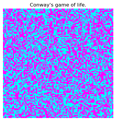
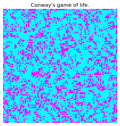
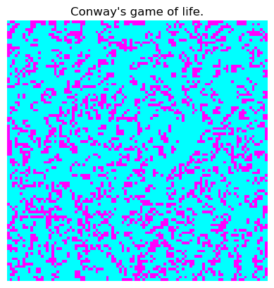
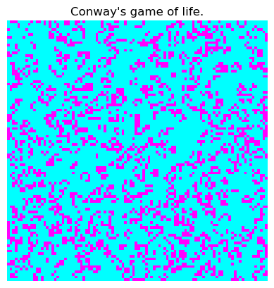
Conclusions
In this notebook we explore:
- Introduction
- Zen of Python
- Optimization
- Python Syntax I
- Variables
- Data Types
- Mathematical Operations
- Python Syntax II
- Containers
- Loops
- Conditionals
- Python Syntax III
- Functions
- Python Syntax IV
- Classes
- Differences between Python 2.x and 3.x
- Integer division
Acknowledgments and References
This Notebook has been adapted by Guillermo Avendaño (WVU), Jose Rogan (Universidad de Chile) and Aldo Humberto Romero (WVU) from the Tutorials for Stanford cs228 and cs231n. A large part of the info was also built from scratch. In turn, that material was adapted by Volodymyr Kuleshov and Isaac Caswell from the CS231n Python tutorial by Justin Johnson (http://cs231n.github.io/python-numpy-tutorial/). Another good resource, in particular, if you want to just look for an answer to specific questions is planetpython.org, in particular for data science.
Changes to the original tutorial include strict Python 3 formats and a split of the material to fit a series of lessons on Python Programming for WVU’s faculty and graduate students.
The support of the National Science Foundation and the US Department of Energy under projects: DMREF-NSF 1434897, NSF OAC-1740111, and DOE DE-SC0016176 is recognized.


Back of the Book
plt.figure(figsize=(3,3))
n = chapter_number
maxt=(2*(n-1)+3)*np.pi/2
t = np.linspace(np.pi/2, maxt, 1000)
tt= 1.0/(t+0.01)
x = (maxt-t)*np.cos(t)**3
y = t*np.sqrt(np.abs(np.cos(t))) + np.sin(0.3*t)*np.cos(2*t)
plt.plot(x, y, c="green")
plt.axis('off');
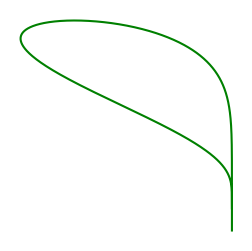
end = time.time()
print(f'Chapter {chapter_number} run in {int(end - start):d} seconds')
Chapter 1 run in 24 seconds
Key Points
Python is an easy-to-learn programming language.