Introduction to Modern Fortran
Overview
Teaching: 60 min
Exercises: 0 minQuestions
What is Fortran?
Why learn Fortran?
Which version of Fortran should I learn?
Objectives
Learning the basic elements of the language
Make the distinction between the older and newer ways of programming in Fortran
Be able to write small and moderate-size codes
The Fortran Programming Language
Fortran is a programming language with a long history. Originally developed in the 1950s, it was first created in a time before the internet, laptop computers, and desktop computers before computers even have a screen. Fortran was created at a time when computers were almost exclusively designed and operated to carry out numerical operations. Programming in Fortran today is very different from how programmers introduce instructions and compile codes. During the first decades of electronic computers, programming was done with punched cards, data was stored in tapes, and results were printed with dot matrix printers. Over more than 60 years, the language itself has evolved to accommodate new ways of programming, new hardware, new levels of complexity, and new ways of using computers for numerical calculations.
Evolution of Fortran
The first versions of the language introduce many of the concepts used today in most programming languages, the idea of loops, conditionals, and variables. Those elements are so commonplace today that we do not see as anything revolutionary, but FORTRAN was the first language to introduce many of those elements in programming, at least in a way that resemble the ways we program today.
The first milestone in the language was achieved with FORTRAN 77. This standard introduces structured programming and the processing of characters. Structured programming allows us to create larger codes and reuse pieces of code in ways that are easier to understand for a human. FORTRAN 77 was so successful that took more than a decade to reach an agreement over the new milestone. Fortran 90 added array, modular and generic programming. Those elements increase the flexibility of codes to accommodate data in run time instead of requiring constant recompilation when the parameters changed. Modules allow even larger codes to introduce tools to aggregate routines with variables. Fortran 90 left behind some issues that were solved in Fortran 95. Fortran 95 clarify some aspects of the language and was the first to introduce some parallelization techniques (HPF) well before OpenMP and other paradigms proved to be more effective for that. Fortran 2003 was the next big step in introducing Object Oriented Programming in a way that makes sense for scientific computing. The most recent developments in the language come from Fortran 2008 and 2018 which includes native parallel computing in the form of Coarrays.
With such extensive evolution of the language, the standard retained compatibility with previous versions, being far more conservative than other languages. Scientific codes are developed for decades and used even longer. Many of the codes that run today on larger supercomputers were first developed in the 1980s and could have 1 million lines of code or more. If the language specification does not retain some compatibility many of those efforts could be lost or will become attached to older compilers losing the ability to evolve themselves.
The purpose of this lecture is to teach Fortran in the ways and styles in use today. Searching over the internet and you can find many websites teaching Fortran. Some of those sites teach Fortran 90, some teach and show examples in FORTRAN 77, and even mixtures of those. There are a few sites and books that present Fortran 2003 and 2008 but still with code style from older ways. In this lecture we will present how Fortran codes are developed today, we try to use as many Fortran 2003/2008 features as possible, examples use modern style, we completely ignore features that have become obsolete, discouraged and deprecated.
Compiling Fortran code
Before we explore the syntax and structure of the Fortran Programming language we will first learn how to compile any of the examples that will be presented from now on.
A code written in Fortran is a text file. A programming language has a strict syntax for the text file needs to follow so the compiler can produce an executable binary.
As an example, we will use a relatively small code. This code implements a simple algorithm that computes pi. We will use an integral formula for pi:
 Integral used to converge pi
The integral will be computed by diving the range into N pieces and computing the rectangles associated to each of them. Assuming a uniform partition in the domain, the quadrature can be computed as:
where
is some point in the interval of the rectangle. In the implementation below we are using the middle point.
The source code is the file (example_00.f90)
program converge_pi

   use iso_fortran_env

   implicit none

   integer, parameter :: knd = max(selected_real_kind(15), selected_real_kind(33))
   integer, parameter :: n = huge(1)/1000
   real(kind=knd), parameter :: pi_ref = 3.1415926535897932384626433832795028841971_knd

   integer :: i
   real(kind=knd) :: pi = 0.0, t

   print *, 'KIND      : ', knd
   print *, 'PRECISION : ', precision(pi)
   print *, 'RANGE     : ', range(pi)

   do i = 0, n - 1
      t = real(i + 0.5, kind=knd)/n
      pi = pi + 4.0*(1.0/(1.0 + t*t))
   end do

   print *, ""
   print *, "Number of terms in the series : ", n
   print *, "Computed value : ", pi/n
   print *, "Reference vaue : ", pi_ref
   print *, "ABS difference with reference : ", abs(pi_ref - pi/n)

end program converge_pi
We will compile this code using 3 different compilers, GCC 11.1,
Load the following modules to access all those 3 compilers
$> module load lang/gcc/11.1.0 lang/nvidia/nvhpc compiler/2021.2.0
Loading these modules we will get access to gfortran, ifort and nvfortran, the names of the Fortran compilers from GNU, Intel and NVIDIA respectively.
The code above can be compiled with each compiler executing:
$> gfortran example_00.f90
$> ifort example_00.f90
$> nvfortran example_00.f90
When compiling the code with any of these compilers a binary file will be created.
The name of the file is by default a.out.
This is convenient name for quick tests like the examples.
To run the resulting binary, type the name of the binary with a ./.
Otherwise, the shell will try to search for a command in the $PATH resulting on an error.
$> ./a.out
You can also compile declaring the name of the final executable, for example using gfortran:
$> gfortran example_00.f90 -o pi
The name of the executable will be pi and can run.
$> ./pi
KIND      :           16
PRECISION :           33
RANGE     :         4931

Number of terms in the series :      2147483
Computed value :    3.14159265358981130850975669310991368
Reference vaue :    3.14159265358979323846264338327950280
ABS difference with reference :    1.80700471133098304108856024329067224E-0014
Elements of the Language
Fortran uses the 26 characters of the English alphabet plus the digits plus a set of characters such as parenthesis, comma, colon, and a few others. This restriction contrast with languages such as Julia that allow basically any UTF-8 string to be a valid variable name (including smile face, greek letters and Chinese ideograms). In Fortran syntax, lowercase letters are equivalent to uppercase, except when they are part of a character string.
In the old style of writing Fortran code that was customary with FORTRAN 77 and before, code was written in UPPERCASE. A good style today consists in writing all the Fortran keywords in lowercase and use uppercase only for elements that are beyond the language itself such as preprocessor directives or directive-based parallelisms such as OpenMP and OpenACC.
There are 4 concepts in the structure of a Fortran code: lexical token, statement, program unit, and the executable program.
Lexical tokens are the keywords, and names. labels, constants, operators and separators. Each token has a particular meaning. Tokens are separated by spaces and the number of spaces does not matter. Some tokens such as parenthesis and operators can be used to separate tokens. We will see this better with examples in our first codes. The spacing between tokens is optional, for example, “end do” and “enddo”. A good coding style will prefer those tokens separated. Most cases where token separation is optional are with “end” and some other keywords like “do”, “function”, “procedure”, “subroutine”, “block”, “if” “program” and others.
In Fortran, the code is written in a text file whose lines can have up to column 132. In the old days of Fortran, the first six columns have a defined use. Today that is obsolete, you can start statements on the first line. Comments can be made with an exclamation mark and all the characters after it will be ignored by the compiler. Example of one statement with comments
! This is the solution to the quadratic equation
y = (-b + sqrt(b**2 - 4*a*c))/(2*a)  ! Notice the need of parenthesis
For long statements you can use up to 255 continuation lines
A single statement can be span across multiple lines using ampersand (&) as the last character.
The continuation line goes to the next first character in the next line, if you use another & the continuation starts in the next character after it. Example (example_01.f90):
program main

   ! This is pi defined as a constant
   ! Most decimals will be ignored as the default precision
   ! for a single precision real data type only provides 6 to 9
   ! significant decimals
   real, parameter :: pi = 3.14159265358979323846264338327950288419716&
                          &9399375105820974944592307816406286208998628&
                          ! This comment works here and does not interrupt
                          ! the continuation line
                          &0348253421170679821480865132823066470938446&
                          ! In standard Fortran 77, anything
                          ! beyond column 72 is ignored.
                          ! In modern Fortran the limit is 132 allowing very long lines like this one
                          &09550582231725359408128481117450284102701938521105559644622948954930381964428810975665933446128475648233&
                          ! Also comments does not count to the limit of 255 continuation lines.
                          &786783165271201909145648566923460348610454326648213393607260249141273

   print *, pi

end program
Multiple statements can be on one line using semicolon (;)
a = 1; b = 2; c = 3
It is not a good style to have long statements on a single line.
types
Fortran define and operate with various types.
The number 3.14 is a floating point number and this is a constant
and you can define a variable pi = 3.14 and pi will also be a floating point number.
Both variables and constant store data. In variables the value they hold can change over the course of a program. You can operate with variables and constants on the same statement, for example:
pi - 3.0
Fortran contains 5 intrinsic types: character, integer, real, logical and complex.
For each intrinsic type, we can consider variations of them, they are called kind and a non-negative integer is used to differentiate each variation.
Different from the common usage, there is nothing in the standard that the integer means the number of Bytes to store the type.
You can build extra types as combinations of those intrinsic types. They are called derived types. Multiple elements of the same type can be arranged in what is called an array
integer
On a computer using 32 bits for representing integers, the range of values is:
As those ranges varied between machines and compilers it is better to ask for a kind that is able to support the values that we declare. In the example below to store numbers up to six digits:
integer, parameter :: i6 = selected_int_kind(6)
And number can be declared as
123456_i6.
-9_i6
We will discuss a variable declaration and intrinsic functions.
The point to make here is that we can control the kind of constant or variable by asking for the right kind that supports the range of interest.
real
The real type stores truncated real numbers. As the internal representation of a number is binary a number such as 1.5 or 1.25 has a exact representation using the real type. A number such as 0.1 will never be exactly represented no matter how many bits you use to represent it. The number 0.1 in binary is:
0.00011001100110011001100110011001100110011001100110011...
A type real number is only able to store a truncated representation of a number. A few numbers can be represented exactly but almost every real number needs to be truncated. Mathematically, the number of real numbers that can be exactly represented with N bits has a Lebesgue measure of zero.
Numbers of real type are stored using some bits for the exponent and some bits for the mantissa and a couple of bits for the sign of mantissa and exponent.
Same as we have for integers, we can ask for the kind that supports a given range of values, using:
integer, parameter :: r9 = selected_real_kind(9, 99)
In this case we are asking for the right kind to store a number with 9 significant decimal digits and between -99 and 99 for the decimal exponent. You can ask for a literal constant to be of that kind using
1.1_r9
9.1E30_r9
Contrary to some common belief, the Fortran Standard does not force a particular number of bit for exponent or mantissa. Compilers abide by the IEEE standard for floating point numbers will a range of [-37:37] for the decimal exponent and about 6 significant digits.
There are functions to inquire about the kind, number of significant decimals, and the range of exponents using the functions:
program main

   integer, parameter :: r9 = selected_real_kind(9, 99)

   print *, 'Information about : selected_real_kind(9, 99)'
   print *, 'KIND      : ', kind(1.1_r9)
   print *, 'PRECISION : ', precision(1.1_r9)
   print *, 'RANGE     : ', range(1.1_r9)

end program
The answer in gfortran on a x86_64 machine is:
 Information about : selected_real_kind(9, 99)
 KIND      :            8
 PRECISION :           15
 RANGE     :          307
Notice that we got 8 as the kind.
In the case of gfortran any many compilers the kind returned 8.
This number is corresponds to the number of bytes used to store the number, but that should not be assume to be 8 on a different compiler.
Notice that the values of precision and range returned are larger than the requested.
The function selected_real_kind will return a kind that meets or exceeds the expectations in terms of precision and range.
In some codes you can see variables being declared as REAL*8 or DOUBLE PRECISION.
Those are valid but discouraged syntax.
You should always use the kind to declare specific variants of an intrinsic type.
complex
Fortran, being a code for scientific computation, has natural support for complex numbers. Complex numbers are built from two numbers, you can declare a complex number with integers or real numbers. The internal representation will be real and of the greatest kind between the real and imaginary parts.
character
A string of characters for literal constants can be defined using single or double quotes (example_03.f90).
program main

   print *, "Using literal with double quotes, I can print ' "
   print *, 'Using literal with single quotes, I can print " '

   !print *  ` Grave accents are not valid quotes`
   !print *, ``No matter how many you use``

   print *, ""
   print *, "Lorem ipsum dolor sit amet, consectetur adipiscing elit,  &
           &       sed do eiusmod tempor incididunt ut labore et       &
           &       dolore magna aliqua. Ut enim ad minim veniam, quis  &
           &       nostrud exercitation ullamco laboris nisi ut aliquip&
           &       ex ea commodo consequat. Duis aute irure dolor in   &
           &       reprehenderit in voluptate velit esse cillum dolore &
           &       eu fugiat nulla pariatur. Excepteur sint occaecat   &
           &       cupidatat non proident, sunt in culpa qui officia   &
           &       deserunt mollit anim id est laborum."


end program main
When coping code from the a webpage, sometimes, you get strings using the grave accent (`).
This kind of quote is not valid and will fail during compilation.
logical
The last type of literal constant is the logical type.
Values can be .true. or .false.
Names
Fortran is extremely flexible for creating names for entities inside a program.
Different from other languages, there are no reserved words in the language.
This a valid, but terrible way of naming variables (example_04.f90)
program main

   integer :: program = 1
   real :: real = 3.14
   character :: print = 'this'

   print *, program
   print *, real
   print *, print

end program
The only rule is that a name must start with a letter and consist only of alphanumeric characters without spaces. Out a this minimal rule, the programmer has a lot of freedom to choose names. Some common sense guidelines for choosing names are:
- Use names with some meaning, except for dummy indices like i, j, k, n and m.
- Names with multiple characters are easy to search on a text editor.
- Too long names are hard to write and prone to typos.
- Link multi-word names with underscores like
electron_densityor use camel case likeElectronDensity. - Remember that Fortran is insensitive to case and that includes names, so
electron_densityandElectron_Densityare the same.
Variables
We have use variables before and we will formalize the structure.
Example (example_05.f90)
program main

   integer(kind=4) :: i = 9, j
   real(kind=8) :: x = 3.14, y, z
   complex(kind=4) :: sec = (-1, 1)
   character(len=20, kind=1) :: word = "Electron"
   logical(kind=1) :: is_good, is_bad

   print *, 'Integer   : ', i
   print *, 'Real      : ', x
   print *, 'Complex   : ', sec
   print *, 'Character : ', word
   print *, 'Logical   : ', is_good

end program
We are using numbers for the kinds for simplicity. Remember that those are not standard and should not be used assuming certain values. Each statement declaring a variable has the name of the type, optionally in parenthesis the kind and in the case of characters, the length and the kind. Two colons separate a list of variables separated by coma and initial values given on the same statement.
Derived types
Beyond the 5 intrinsic types, you can create your own types by grouping several other types intrinsic or not inside what is called a derived type
This example shows how to create, instantiate (create structure) and access the internals of a derived type (example_06.f90):
program main

   type position
      real :: x, y, z
   end type position

   type atom
      character(20) :: atom_name
      character(3)  :: symbol
      integer       :: atom_Z
      real          :: electronegativity
      type(position):: atom_pos
   end type atom

   type(atom) :: gold = atom('Gold', 'Au', 79, 2.54, position(1.0, -1.125, 3.5))

   gold%atom_Z = 79

   print *, 'Name       : ', gold%atom_name
   print *, 'Z          : ', gold%atom_Z
   print *, 'Position Z : ', gold%atom_pos%z

end program
In the example above, atom is a derived type.
atom_name, symbol, atom_Z and electronegativity
are components of the atom type.
atom_pos is also a component and it is itself a derived type.
The variable gold is a structure of the atom type.
For initializing gold we used the type constructor atom('Gold', 'Au', 79, 2.54, position(1.0, -1.125, 3.5)) and the position itself was constructed.
The percentage (%) symbol is a component selector for the internal pieces an atom type.
If the component is also a derived type more (%) are used for the internal structures of the variable.
Despite a complex being an intrinsic variable, it uses the percentage (%) to access the pseudo components re and im.
Arrays
Arrays is one of strengths of the Language. Many other programming languages such as Matlab and Python, took inspiration from Fortran to express complex descriptions of data in arrays.
An array is a uniform arrangement of elements of the same type and type parameters. Arrays can have one or more dimensions. The dimension is established with the attribute dimension. The language imposes a limit of 15 dimensions which is more than is practical today. An array with 15 dimensions and 10 elements on each dimension will require almost 1 PB of memory.
Different from other languages such as C or Python, by default array indices, start in 1. The bounds of a Fortran array can be defined as arguments of the attribute dimension. The number of dimensions of an array is called rank. The number of elements on each dimension is called extent The sequence of extends for all the dimensions is called the shape
The way data is stored for an array is extremely important for computational performance.
An array
real, dimension(3,3) :: a
has the following contiguous Elements
a(1,1) a(2,1) a(3,1) a(1,2) a(2,2) a(3,2) a(1,3) a(2,3) a(3,3)
When we discuss loops on arrays the internal faster loop must run over the internal most contiguous index. This is the complete opposite of the way a language like C represents multidimensional arrays.
Sections of arrays can be referenced using the colon notation a(i:j), where elements in indices i up to jis returned. Array sections
cannot be sectioned again.
Constructors
Array constants can be defined in two notations.
a = (/ 1, 2, 3, 4, 5, 6, 7, 8 /) ! Old Notation
b = [ 2, 4, 6, 8, 10, 12, 14, 16 ]   ! Fortran 2003 notation
There are constructors for constant arrays using implicit loops. The arrays
a = (/ (i, i=1, 8) /)
b = [ (i, i=2, 16, 2) ]
Allocatables
One of the big innovations of Fortran 90 was the inclusion of Dynamic memory allocation via the attribute allocatable for arrays.
Before memory allocation, programmers create arrays of predefined size, sometimes overestimating the size of the array or demanding recompilation to adjust the size of arrays to different problems.
An allocatable array is defined like this:
real, dimension(:, :), allocatable :: a
When the variable is first created it is in unallocated state.
Allocation and deallocation are done with the allocate and deallocate
allocate(a(n,-m:m))
...
deallocate(a)
Strings of characters
There is a special way of declaring strings of characters.
character(len=34) :: name
Despite of being formally different from an array of characters many of the notation for addressing elements and extracting portions of arrays hold for strings
Pointers
A variable that refers to other variable is called a pointer. Pointers are powerful means of declaring operations that apply to different elements using a notation that uses those pointers to as the name says, point to a different variable each time.
Declaration is as follows:
integer, pointer :: pn
real, pointer    :: px
real, pointer, dimension(:,:) :: pa
What happens behind curtains is that each of those variables use a portion of memory to contain a descriptor, that holds not only the memory location, but also the type, and in the case of arrays, bounds and strides.
When a pointer is created, it is by default undefined, i.e there is no way to know if they point something. A pointer can be nullified with:
real, pointer :: px => null()
This is the recommended way of creating pointers as the state can be determined. During the code, the code can point to other variables and can be null again with:
nullify(pa, px)
Expressions and Statements
Variables and constants interact with each other via operators. For example when you write:
c = b + 5
You are using the dyadic operator plus (+) and use the variable b and constant 5.
The result of that operation is assigned ie stored in the memory associated to c.
Most operators are dyadic but there are also monadic operators such as minus (-) when used isolated.
Expressions without parentheses are evaluated successively from left to right for operators of equal precedence, except for exponent ** that is operated first.
For example
f = a/b/c/d
Is actually computed as a/b then the result divided by c and finally the result divided by d. At the end of calculation, the final value is assigned to f
This operation can be actually be computed as
f = a/(b*c*d)
As compilers could identify that divisions are more computationally expensive than multiplications and prefer a single division.
For exponents the evaluation is right to left, for example a**b**c is evaluated as a**(b**c)
Division between integers return integer, the value truncated, not rounded example:
12/3  is 4
14/3  is 4
When numbers of different type operate the return is for the stronger type and the weakest type is promoted before operation.
Numerical variables can be promoted to different type using functions
| Type | Convertion Fuction |
|---|---|
| integer | int(expr, kind(variable)) |
| real | real(expr, kind(variable)) |
| complex | compl(expr, kind(variable)) |
You can use the same function to change inside the same type but different kind.
Operators that return boolean
| Operator | Description |
|---|---|
| < | Less than |
| > | Greater than |
| <= | Less than or equal |
| >= | Greater than or equal |
| == | equal |
| /= | not equal |
Booleans themselves receive operators:
| Operator | Description |
|---|---|
| .not. | logical negation |
| .and. | logical intersection |
| .or. | logical union |
| .eqv. | logical equivalent |
| .neqv. | logical non-euivalent |
Array Expressions
Operations over arrays are greatly simplified by using the concept of conformable arrays. Two arrays are conformable if the have the same *shape, ie, the same dimension, and the same number of elements on each dimension. The actual indices can differ. Scalars are conformable to any array and the value will operate one-to-one over each element of the array.
Consider an array:
real, dimension(30,10) :: a, b
real, dimension(10) :: v
The following operations are valid
a/b      ! Array with shape [30,10] with entries a(i,j)/b(i,j)
b+3.14   ! Array with shape [30,10] with values b(i,j)+3.14
v + b(11:20, 10) | Array with shape [10]
a == b   ! Boolean comparison, .true. if all individual comparisons are true
Control Constructs
Programs with just a linear sequence of statements cannot produce the right flow of instructions needed even by a simple algorithm. Control constructs are build with blocks, some keyword at the very beginning and a final end … at the end. Control constructs can be nested and a outer block cannot end before all nested blocks are also ended.
There are two major sets of controls.
Those that diverge the execution based on an expression being true or false.
These kind of controls are called conditionals.
The typical conditional in Fortran is the if _expression_ else _statements_ end if
There are also controls that repeat the contents of a block a certain number of times or until a condition is reached.
Those are called loops.
The usual loop in Fortran is the do statements end do
Conditional if
The conditional if is used when the execution can go to at most one case.
It could do nothing or having more test conditions, but only one block will be executed. Conditional as any block can be named:
The following example is good fore reference:
posneg: if (x > 0) then
  print *, 'Positive number'
else if (x < 0 ) then
  print *, 'Negative number'
else
  print *, 'Value is zero'
end if posneg
The conditional has a name (posneg) and this is optional.
The else if and else are optional too.
The else clause in case it exists, must be the final clause.
For very quick conditional there is one line form that is useful
if (x /= 0) print *, 'Non zero value'
Conditional case
The second conditional in Fortran is case.
In this case, there is only one evaluation but multiple blocks can be executed based on a selector and selector.
There is also an option for a default value that is executed if any of the other cases were.
Example:
select case
   case (:-1)
      x = -1.0
case (0)
      x = -1E-8
case (3:)
      x = 3.14
default
      x = 0.0
end select
Loop do
The do loop has a rich construct that is able to not doing anything to run an infinite loop. do loops is one of the oldest constructs in fortran and have received a lot of variations over different Fortran versions.
For this introductory lesson a simple form is shown. As example consider a simple but not particularly efficient way of computing a matrix multiplication:
do i = 1, n
   do j = 1, m
      a(i,j) = 0.0
      do l = 1, k
         a(i,j) = a(i,j) + b(i,l)*c(l,j)
      end do
   end do
end do
There are two special statements that alter the repetition in do loops.
exit skips entirely the loop and set the program to continue on the first line after end do.
With nested cycles it is possible to abandon an outer loop from an inner loop and we will see this on the advanced hour.
cycle will skip one run and set the execution just before end do, meaning that the next iteration will take place but all the code after the cycle will be skipped.
Consider this simple example:
do c = 1, 100
  dis = b**2 - 4*a*c
  if dis < 0 exit
end do
Programs, Procedures, and Modules
A program is composed of a set of variable definitions, assignments, statements, and control blocks such as loops and conditionals. All those pieces of code are organized into programs, procedures, and modules.
This is a brief review of each of them and will provide the bare minimum to start writing simple programs on your own.
Any program has at least one main program. We have already used one for our first example. The basic structure of the main program is
program name

! variable definitions
...

! statements
...

end program
Writing an entire code in a single program is possible but will produce a code with a lot of redundancy and very hard of maintain.
The next level of complexity is to take pieces of code and convert them in procedures.
There are two kinds of procedures: A function and a subroutine
The difference is that functions return a single value and usually does not alter the input (at least to be aligned to the concept of mathematical function).
A subroutine does not return anything so it cannot be included as part of an expression, but it can change the arguments, effectively giving a mechanism to alter the state of the variables and the calling program.
A subroutine is called using the clause call
The next level is to group procedures, functions and types into a coherent structure called modules. Modules are powerful way of structuring large codes. Even small codes benefit from modules as they offer type checking that internal procedures will not offer.
Some examples will clarify these concepts needed for the exercises proposed later on.
A very minimal program will be something like this:
program test
   print *, ’Hello world!’
end program test
This program has just one statement, no variables, no calls to subroutines or functions. This program itself written in a file can be compiled and the code executed. See the first section of this lesson where we show how to compile a code like this.
Apart from the program, there are subprograms, their structure is very similar to the main program but the resulting code can only be called from other programs or subprograms.
A subroutine is defined as
subroutine sub(a, x, y)
   real, intent(in) :: a
   real, intent(in), dimension(:) :: x
   real, intent(out), dimension(:) :: y

   y = a*x

end subroutine
The subprogram function is similar to subroutines but they can be called on expressions and typically will not change the arguments.
One example:
function distance3D(p1, p2)

  real :: distance = 0.0
  real, intent(in), dimension(3) :: p1, p2
  integer :: i

  do i=1, 3
    distance = distance + (p1(i)-p2(i))**2
  end do

  distance = sqrt(distance)

end function distance3D
Input and Output
Such short introduction to the language will inevitably leave several topics completely uncovered. Input/Output is a quite complex topic for such short lecture.
What follows is just the bare minimum for producing rudimentary but effective output on the screen and receiving input from the keyboard or command line.
We have use the print clause, it is quite simple to use like this:
print *, 'VAR 1: ', var1, 'VAR2: ', var2
This clause will print on the standard output, which by default the shell associate to the terminal.
Command Line Arguments
One of the novelties of 2003 is to allow Fortran programs to read from the command line.
Consider this example (example_10.f90)
program main

   implicit none

   integer :: i
   character(len=1024) :: arg
   integer :: length, istatus

   print *, 'Number of arguments', command_argument_count()

   do i = 1, command_argument_count()

      call get_command_argument(i, arg, length, istatus)

      print *, trim(arg)

   end do

end program
The arguments are strings but can be converted using the read function.
Example (example_11.f90):
program main

   implicit none

   integer :: i
   character(len=1024) :: arg
   integer :: length, istatus
   real :: a(3)

   print *, 'Number of arguments', command_argument_count()

   do i = 1, command_argument_count()

      call get_command_argument(i, arg, length, istatus)

      print *, trim(arg)

   end do

   if (command_argument_count() == 3) then

      do i = 1, 3
         call get_command_argument(i, arg, length, istatus)
         read (arg, *) a(i)
      end do

   end if

   print '(3(e12.3))', a(:)

end program
Key Points
Fortran is one of the oldest programming languages still in active use
Many important scientific codes are written in Fortran
Fortran is a Programming Language especially suited to High-Performance numeric computation
Fortran has evolved over the years adding and removing features to accommodate the evolution of scientific computing
Fortran is a very expressive language when dealing with arrays
Using Fortran modules facilitate the creation of large software projects
Best Practices in Modern Fortran
Overview
Teaching: 60 min
Exercises: 0 minQuestions
How to move out of Fortran 77 into Modern Fortran styles?
Objectives
Learn the difference between deprecated styles and the modern ways of Fortran coding.
Best Practices in Modern Fortran
Fortran is a language with a long history. Fortran is one of the oldest Programming Languages still in active use. That old history means that the language has evolved in expression and scope over more than 60 years.
The way you programmed Fortran back in the 60s, 70s, and 80s is completely inadequate for modern computers. Consider for example the length of the lines. Back in the 70s and 80s, people programmed computers using punched cards and later dumb terminals connected to mainframes. Those terminals have a limited number of characters in one line. It is from that time that a limit of 72 characters on one line and characters beyond column 72 were ignored. The first five columns must be blank or contain a numeric label. Continuation lines were identified by a nonblank, nonzero in column 6. All these limitations were present in what is called the Standard Fixed Format of Fortran 77.
Over time, these limitations and many others in the language became obsolete but were still in use for decades even after Fortran 90 was the new Standard. Back in the 90s, there were no free Fortran 90 compilers, people continue to use Fortran 77 with restrictions relaxed and some characteristics of Fortran 90 were integrated little by little into the compilers.
The fact is that there are many codes written in Fortran 77. If you search for Fortran tutorials and documentation, there are many pages in academics that still teach Fortran 77. Fortran 90 was gaining space and later Fortran 95. Today almost main Fortran compilers support Fortran 2003 entirely and Fortran 2008 to a fairly complete degree. New features in Fortran 2018 are still not implemented in the latest version of major compilers.
In previous sections, we have discussed the basic elements so you can read and write code in Fortran. We learn about variables assignments subroutines and modules and we explored those elements using the modern ways of writing code in Fortran. In this section we will have to learn a bit about the “old ways” in such a way that when you encounter those pieces of code, you can recognize them knowing which are the alternatives and best practices used today. This is in this way an intermediate class in Modern Fortran. I assume you know the basics and are able to write useful code in Fortran. The idea is to recognize old Fortran 77 and Fortran 90 styles and be able to translate those into modern Fortran 2003 and 2008 Standards. By doing that you are moving the code into more flexible, readable, extensible, and potentially with more performance.
The old Fortran 77
Fortran 77 was a powerful language back in its time.
It was so powerful that stay as the standard de facto well in the 90s.
Many elements of the language still in use today were added to Fortran 77 to address the limitations of FORTRAN 66.
For example the IF and END IF statements including ELSE and ELSE IF were the first steps into structured programming.
These statements were an important move to move GOTO into oblivion.
GOTOwas one of the reasons why codes were so difficult to follow and almost unpredictable when were the source of a bug.
Another powerful element of the language were intrinsic functions such as SQRT that accept complex or double precision numbers as arguments.
All these niceties today are taken for granted but back then were big improvements to the language.
However, the language has important flaws.
One important is the lack of dynamic memory allocation.
The code still promotes a code that is cluttered, with missing blanks, and in general hard to read.
Now the question is if a code works in Fortran 77 why change it? Investing some time now in rewriting a code in a new language could return in big gains later on. A new structure could emerge that uses better memory (with dynamic allocation) to structure the code in ways that make it easier to read and extend. There are good reasons and rewards for better and cleaner code.
Free Format
Back to the first versions of Fortran, the first 5 columns of characters were dedicated as label fields. A C in column 1 means that the line was treated as a comment and any character in column 6 means that the line was a continuation of the previous statement.
Today those restrictions are no longer needed.
Statements can start in the first column.
An exclamation mark starts a comment and comments could be inserted any place in the line, except literal strings.
Blanks help the readability of the code.
Variables cannot have spaces, it is a better practice to use underscore for multi-word variables.
Use & as the last character for continuing on the next line.
Declaring multiple statements on the same line is possible with a semicolon (;) but use it only for very short statements.
Example (example_01.f90):
program free_form
   print *, 'This statement starts in column 4 (with indentation)'
   x = 0.1; y = 0.7 ! Two small statements in one line
                    ! Comment with an exclamation mark
   tan_x_plus_y = tan(x) + tan(y) / &  ! Line with continuation
           (1- tan(x)*tan(y))
end program free_form
Use blank characters, blank lines and comments to improve the readability of your code. A cluttered code is hard to read and you are not doing any good trying to fit most of your code in one screen page.
Instead of this (example_02_bad.f90):
!BAD CODE
program log_sqrt
x=99.9
y=log10(sqrt(x))
if(y.lt.1.0) print *,'x is less than 100'
end program
This code is too compact, it is not hard to read because is too small, but for bigger codes became really hard to follow.
An alternative is like this (example_02_bad.f90):
!GOOD
program log_sqrt

   x = 99.9
   y = log10(sqrt(x))

   if (y .lt. 1.0) &
           print *, 'x is less than 100'

end program log_sqrt
We include spaces to clarify variable assignments from the conditional.
Indentations inside the program and end program also help to visualize the scope of blocks.
Old style DO loops
In old FORTRAN 77, do loops have a numerical identifier to jump to a continue statement to cycle the loop, that is completely obsolete and must be avoided in modern coding (example_03_bad.f90):
      PROGRAM square
      DO 100 I=1,100
      X=I
      X2=X*X
      IF(X2.LT.100) print *, 'X=', I, ' X^2 will have less than 3 digits
100   CONTINUE
      END
This old style of coding wastes 6 columns of space, uses a labeled statement for cycling and is written with full capitalization.
An alternative is something like this (example_03_good.f90):
program square

   implicit none

   real :: x, x2
   integer :: i

   do i = 1, 100
      x = i
      x2 = x*x
      if (x2 < 100) &
         print *, 'X=', I, ' X^2 will have less than 3 digits
   end do

end program
This code uses indentations and has an end do that is clearer for the user when the loops grow or became nested. We will discuss the implicit down below
Variable Attributes
Fortran 95 introduce variable attributes and they were extended in Fortran 2003 and 2008. The most common attributes are
parameter, dimension, allocatable, intent, pointer, target, optional, private, public, value and bind
From those, we will demonstrate the first 3.
parameter is important for declaring constants that otherwise will require going beyond the language and using the preprocessor.
dimensionis used to define the length of arrays or the dimension using colons and commas to declare it.
allocatable is used for the dynamic allocation of arrays an important feature introduced in Fortran 90 and expanded in Fortran 95 and beyond.
This is an example using these 3 attributes that should be frequently used (example_04.f90).
program f95attributes

   implicit none

   integer :: i, j
   integer, parameter :: n = 100
   real :: x
   real, parameter :: pi = 3.141592653
   real, dimension(n) :: array
   real, dimension(:, :), allocatable :: dyn_array2d

   allocate (dyn_array2d(2*n, 2*n))

   do i = 1, 2*n
      do j = 1, 2*n
         dyn_array2d(j, i) = j + 0.0001*i
      end do
   end do

   do i = 1, 10
        print '(10(F9.4))', dyn_array2d(i,1:10)
   end do

end program
implicit none
By default all variables starting with i, j, k, l, m and n are integers.
All others are real.
Despite of this being usually true for small codes, it is better to turn those defaults off with implicit none
Variables in large codes will have names with scientific meaning and the defaults can bring bugs that are hard to catch.
program implicit
   ! use to disable the default
   implicit none

   real :: J_ij !Interaction factor in Ising Model

end program
Loops, exit and cycle
Use exit to abandon a loop and cycle to jump to the next iteration.
These are better replacements to complicated GOTO statements from old FORTRAN.
You can use exit and cycle in bounded and unbounded loops.
The file example_05.f90 and example_06.f90 show the effect of exit and cycle respectively.
program do_exit

   implicit none

   integer :: i
   real, parameter :: pi = 3.141592653
   real :: x, y

   do i = 0, 360, 10
      x = cos(real(i)*pi/180)
      y = sin(real(i)*pi/180)

      if (abs(x) < 1E-7) then
         print *, "Small denominator (exit)"
         exit
      end if
      print *, i, x, y, y/x
   end do

   print *, 'Final values:', i, x

end program
program do_cycle

   implicit none

   integer :: i
   real, parameter :: pi = 3.141592653
   real :: x, y

   do i = 0, 360, 10
      x = cos(real(i)*pi/180)
      y = sin(real(i)*pi/180)

      if (abs(x) < 1E-7) then
         print *, "Small denominator (cycle)"
         cycle
      end if
      print *, i, x, y, y/x
   end do

   print *, 'Final values:', i, x

end program
In the case of nested loops, the solution is to name the loop.
Constructs such as do, and if as case can be named and you can use the name to leave outer loops from inside an inner loop.
...
outer: do i = 0, 360, 10
   inner: do j = 0, 360, 10
      x = cos(real(i)*pi/180)
      y = sin(real(j)*pi/180)

      if (abs(x) < 1E-7) then
         print *, "Small denominator (exit)"
         exit outer
      end if
      print *, i, x, y, y/x
   end do inner
end do outer
...
...
outer: do i = 0, 360, 10
   inner: do j = 0, 360, 10
      x = cos(real(i)*pi/180)
      y = sin(real(j)*pi/180)

      if (abs(x) < 1E-7) then
         print *, "Small denominator (cycle)"
         cycle outer
      end if
      print *, i, x, y, y/x
   end do inner
end do outer
...
The case construct
The case construct in Fortran works different from its homologous in C language.
In C you need to use a break, otherwise the code will test every single case.
In Fortran once one case passes the condition, the others will be skipped.
In Fortran case take ranges apart from a single element as other languages.
Example:
integer :: temp_gold

! Temperature in Kelvin!
select case (temp_gold)
case (:1337)
write (*,*) ’Solid’
case (1338:3243)
write (*,*) ’Liquid’
case (3244:)
write (*,*) ’Gas’
case default
write (*,*) ’Invalid temperature’
end select
The kind of variables
There are at least 2 kinds of reals: 4-byte, 8-byte. Some compilers offer the third kind with 16-byte reals. The kind numbers are usually 4, 8, and 16, but this is just a tradition of several languages and not mandatory by the language. The kind values could be 1, 2 and 4.
There is an intrinsic module called iso_fortran_env that provides the kind values for logical, character, integer, and real data types.
Consider this example to get the values used (example_07.f90)
program kinds

   use iso_fortran_env

   implicit none

   print *, 'Logical  : ', logical_kinds
   print *, 'Character: ', character_kinds
   print *, 'Integer  : ', integer_kinds
   print *, 'Real     : ', real_kinds

end program kinds
Different compilers will respond with different kinds values.
For example, gfortran will return this:
Logical  :            1           2           4           8          16
Character:            1           4
Integer  :            1           2           4           8          16
Real     :            4           8          10          16
As Fortran have evolve over the years, several ways were created to declare the storage size of different kinds and consequently the precision of them. This example explores some of those old ways that you can still encounter in codes.
Consider this example illustrative of the multiple ways of declaring REAL variables (example_08.f90):
program kinds

   use iso_fortran_env

   implicit none

   integer :: i, my_kind

   real :: x_real              ! the default
   real*4 :: x_real4           ! Real with 4 bytes
   real*8 :: x_real8           ! Real with 8 bytes
   DOUBLE PRECISION :: x_db    ! Old way from FORTRAN 66

   integer, parameter :: k9 = selected_real_kind(9)
   real(kind=k9) :: r

   print *, 'Kind for integer            :', kind(i)
   print *, 'Kind for real               :', kind(x_real)
   print *, 'Kind for real*4             :', kind(x_real4)
   print *, 'Kind for real*8             :', kind(x_real8)
   print *, 'Kind for DOUBLE PRECISION   :', kind(x_db)
   print *, ''

   my_kind = selected_real_kind(9)
   print *, 'Which is the "kind" I should use to get 9 significant digits?  ', my_kind

   my_kind = selected_real_kind(15)
   print *, 'Which is the "kind" I should use to get 15 significant digits? ', my_kind

   r = 2._k9;
   print *, 'Value for k9', k9
   print *, 'Square root of 2.0 for default real      :', sqrt(2.0)   ! prints 1.41421354
   print *, 'Square root of 2.0 for DOUBLE PRECISION  :', sqrt(2.0d0) ! prints 1.41421354
   print *, 'Square root of 2.0 for numer of kind(k9) :', sqrt(r)     ! prints 1.4142135623730951

end program
The original REAL data type have received multiple variations for declaring floating point numbers based on rather ambiguous terms such as DOUBLE PRECISION which actually does not mean what literally says.
Other variations use the kind assuming that the numbers 4, 8, and 16 represent the number of bytes used by each data type, this is not standard and Salford f95 compiler used kinds 1,2, and 3 to stand for 2- 4- and 8-byte.
Notice that storage size is not the same as precision. Those terms are related and you expect that more bytes will end up giving more precision, but REALS have several internal components such as the size of mantissa and exponent. The 24 bits (including the hidden bit) of mantissa in a 32-bit floating-point number represent about 7 significant decimal digits.
Even though, this is not the same across all the real space. We are using the same number of bits to represent all normalized numbers, the smaller the exponent, the greater the density of truncated numbers. For example, there are approximately 8 million single-precision numbers between 1.0 and 2.0, while there are only about 8 thousand numbers between 1023.0 and 1024.0.
Beyond the standard representation, you can also change the storage size during compilation. Below, the same code was compiled using arguments that change the storage size of different variables.
$> gfortran example_08.f90
$> ./a.out
 Kind for integer            :           4
 Kind for real               :           4
 Kind for real*4             :           4
 Kind for real*8             :           8
 Kind for DOUBLE PRECISION   :           8

 Which is the "kind" I should use to get 9 significant digits?             8
 Which is the "kind" I should use to get 15 significant digits?            8
 Value for k9           8
 Square root of 2.0 for default real      :   1.41421354
 Square root of 2.0 for DOUBLE PRECISION  :   1.4142135623730951
 Square root of 2.0 for numer of kind(k9) :   1.4142135623730951
$> gfortran -fdefault-real-16 example_08.f90
$> ./a.out
 Kind for integer            :           4
 Kind for real               :          16
 Kind for real*4             :           4
 Kind for real*8             :           8
 Kind for DOUBLE PRECISION   :          16

 Which is the "kind" I should use to get 9 significant digits?             8
 Which is the "kind" I should use to get 15 significant digits?            8
 Value for k9           8
 Square root of 2.0 for default real      :   1.41421356237309504880168872420969798
 Square root of 2.0 for DOUBLE PRECISION  :   1.41421356237309504880168872420969798
 Square root of 2.0 for numer of kind(k9) :   1.4142135623730951
$> gfortran -fdefault-real-16 -fdefault-double-8 example_08.f90
$> ./a.out
 Kind for integer            :           4
 Kind for real               :          16
 Kind for real*4             :           4
 Kind for real*8             :           8
 Kind for DOUBLE PRECISION   :           8

 Which is the "kind" I should use to get 9 significant digits?             8
 Which is the "kind" I should use to get 15 significant digits?            8
 Value for k9           8
 Square root of 2.0 for default real      :   1.41421356237309504880168872420969798
 Square root of 2.0 for DOUBLE PRECISION  :   1.4142135623730951
 Square root of 2.0 for numer of kind(k9) :   1.4142135623730951
Fortran 2008 includes standard kinds real32, real64, real128 to specify a REAL type with a storage size of 32, 64, and 128 bits. In cases where target platform does not support the particular kind a negative value is returned.
This example shows the new kind parameters (example_09.f90).
program newkinds

   use iso_fortran_env

   implicit none

   real(kind=real32) :: x32
   real(kind=real64) :: x64
   real(kind=real128) :: x128

   print *, 'real32  : ', real32, achar(10), &
           ' real64  : ', real64, achar(10), &
           ' real128 : ', real128

   x32 = 2.0
   x64 = 2.0
   x128 = 2.0

   print *, 'SQRT(2.0) using kind=real32  :', sqrt(x32)
   print *, 'SQRT(2.0) using kind=real64  :', sqrt(x64)
   print *, 'SQRT(2.0) using kind=real128 :', sqrt(x128)

end program
The storage size of these variables is no longer affected by the compiler arguments used above.
$> gfortran example_09.f90
$> ./a.out
 real32  :            4
 real64  :            8
 real128 :           16
 SQRT(2.0) using kind=real32  :   1.41421354
 SQRT(2.0) using kind=real64  :   1.4142135623730951
 SQRT(2.0) using kind=real128 :   1.41421356237309504880168872420969818
$> gfortran -fdefault-real-16 -fdefault-double-8 example_09.f90
$> ./a.out
 real32  :            4
 real64  :            8
 real128 :           16
 SQRT(2.0) using kind=real32  :   1.41421354
 SQRT(2.0) using kind=real64  :   1.4142135623730951
 SQRT(2.0) using kind=real128 :   1.41421356237309504880168872420969818
You can still change those kinds during compile time using command line arguments -freal-4-real-10, -freal-8-real-10 and similar ones.
$> gfortran -freal-4-real-10 -freal-8-real-10 example_09.f90
$> ./a.out
 real32  :            4
 real64  :            8
 real128 :           16
 SQRT(2.0) using kind=real32  :   1.41421356237309504876
 SQRT(2.0) using kind=real64  :   1.41421356237309504876
 SQRT(2.0) using kind=real128 :   1.41421356237309504880168872420969818
$> gfortran -freal-4-real-16 -freal-8-real-16 example_09.f90
$> ./a.out
 real32  :            4
 real64  :            8
 real128 :           16
 SQRT(2.0) using kind=real32  :   1.41421356237309504880168872420969818
 SQRT(2.0) using kind=real64  :   1.41421356237309504880168872420969818
 SQRT(2.0) using kind=real128 :   1.41421356237309504880168872420969818
Changing kinds during compile time could have unintended consequences, for example using external libraries as could be the case with MPI.
Allocatable arrays
There are two types of memory for a program: The stack and the heap. Scalars and static arrays live in the stack but the size of that space is very limited and some sysadmins and queue systems limit its value even more. Most other variables including allocatable arrays live on the heap.
Before allocatable arrays were part of Fortran 90, Arrays were created with a fixed size.
Programs used arrays with sizes that overestimated the actual needs for storage or require being recompiled every time the size of those arrays changed.
Still, some scientific codes work with fixed arrays and need recompilation before any simulation.
Modern written codes (Since Fortran 90) used allocatable arrays.
Declarations and allocation happen in two steps instead of a single step with fixed arrays.
As allocation takes time, it is not a good idea to allocate and deallocate very often.
Allocate once and use the space as much as possible.
Fortran 90 introduces ALLOCATABLE attributes and allocate and deallocate functions.
Fortran 95 added DIMENSION attribute as an alternative to specifying the dimension of arrays. Otherwise, the array shape must be specified after the array-variable name. For example (example_10.f90):
program alloc_array

   implicit none

   integer, parameter :: n = 10, m = 20
   integer :: i, j, ierror

   real :: a(10)
   real, dimension(10:100, -50:50) :: b
   real, allocatable :: c(:, :)

   real, dimension(:), allocatable :: x_1d
   real, dimension(:, :), allocatable :: x_2d

   allocate (c(-9:10, -4:5))

   allocate (x_1d(n), x_2d(n, m), stat=ierror)
   if (ierror /= 0) stop 'error in allocation'

   do i = 1, n
      x_1d(i) = i
      do j = 1, m
         c(j - 10, i - 5) = j-10 + 0.01*(i-5) ! contiguous operation
         x_2d(i, j) = i + 0.01*j              ! non-contiguous operation
      end do
   end do

   print *,''
   print '(A, 10(F6.2))', 'x_1d:', x_1d(:)

   print *,''
   do j = -9, 10
      print '(A, 10(F6.2))', 'c   :', c(j, :)
   end do

   print *,''
   do i = 1, n
      print '(A, 20(F6.2))', 'x_2d:', x_2d(i, :)
   end do

   deallocate (c, x_1d, x_2d)

end program
Array Allocations: heap vs stack
Static arrays could be allocated on the stack instead of using the heap.
The stack has a limited size and under some circumstances, static arrays could exhaust the stack space allowed for a process.
Consider this example (example_12.f90):
program arraymem

   use iso_fortran_env

   implicit none

   integer, parameter :: n = 2*1024*1024 - 4096

   print *, 'Numeric Storage (bits): ', numeric_storage_size
   print *, 'Creating array N ', n

   call meanArray(n)

contains

   subroutine meanArray(n)
      integer, intent(in) :: n
      integer :: dumb
      integer, dimension(n) :: a
      a = 1
      !print *, sum(a)
      read *, dumb
   end subroutine meanArray

end program arraymem
You can check the limit for stack memory on the machine:
$> ulimit -S  -s
8192
$> ulimit -H  -s
unlimited
We have a soft limit of 8MB for stack and the user can raise its value to an unlimited value.
As the limit is 8MB we will create an integer array that takes a bit under 8MB. The array will be of integers and each integer takes by default 4 Bytes. This is not a safe value but will work for the purpose of demonstrating the effect:
n = 2*1024*1024 - 4096
Now we will compile the code above with gfortran, forcing the static arrays to be on stack.
Some compilers move large arrays to heap automatically so we are bypassing this protection.
$> gfortran -fstack-arrays example_12.f90
$> ./a.out
Sometimes you will get an output like this:
 Numeric Storage (bits):           32
 Creating array N      2093056
Segmentation fault (core dumped)
We are so close to filling the stack that small variations in loading libraries could cross the limit. Try a few times until the code stops when asking for input from the keyboard.
Once the code is waiting for any input, execute this command on a separate terminal:
$> pmap -x `ps ax | grep a.ou[t] | awk '{print $1}' | head -1`
The command pmap will print a map of the memory and the stack is marked there.
Address           Kbytes     RSS   Dirty Mode  Mapping
0000000000400000       4       4       0 r---- a.out
0000000000401000       4       4       0 r-x-- a.out
0000000000402000       4       4       0 r---- a.out
0000000000403000       4       4       4 r---- a.out
0000000000404000       4       4       4 rw--- a.out
0000000001a3e000     132      16      16 rw---   [ anon ]
00007f8fb9948000    1808     284       0 r-x-- libc-2.17.so
00007f8fb9b0c000    2044       0       0 ----- libc-2.17.so
00007f8fb9d0b000      16      16      16 r---- libc-2.17.so
00007f8fb9d0f000       8       8       8 rw--- libc-2.17.so
00007f8fb9d11000      20      12      12 rw---   [ anon ]
00007f8fb9d16000     276      16       0 r-x-- libquadmath.so.0.0.0
00007f8fb9d5b000    2048       0       0 ----- libquadmath.so.0.0.0
00007f8fb9f5b000       4       4       4 r---- libquadmath.so.0.0.0
00007f8fb9f5c000       4       4       4 rw--- libquadmath.so.0.0.0
00007f8fb9f5d000      92      24       0 r-x-- libgcc_s.so.1
00007f8fb9f74000    2044       0       0 ----- libgcc_s.so.1
00007f8fba173000       4       4       4 r---- libgcc_s.so.1
00007f8fba174000       4       4       4 rw--- libgcc_s.so.1
00007f8fba175000    1028      64       0 r-x-- libm-2.17.so
00007f8fba276000    2044       0       0 ----- libm-2.17.so
00007f8fba475000       4       4       4 r---- libm-2.17.so
00007f8fba476000       4       4       4 rw--- libm-2.17.so
00007f8fba477000    2704     220       0 r-x-- libgfortran.so.5.0.0
00007f8fba71b000    2048       0       0 ----- libgfortran.so.5.0.0
00007f8fba91b000       4       4       4 r---- libgfortran.so.5.0.0
00007f8fba91c000       8       8       8 rw--- libgfortran.so.5.0.0
00007f8fba91e000     136     108       0 r-x-- ld-2.17.so
00007f8fbab29000      16      16      16 rw---   [ anon ]
00007f8fbab3d000       8       8       8 rw---   [ anon ]
00007f8fbab3f000       4       4       4 r---- ld-2.17.so
00007f8fbab40000       4       4       4 rw--- ld-2.17.so
00007f8fbab41000       4       4       4 rw---   [ anon ]
00007ffd65b94000    8192    8192    8192 rw---   [ stack ]
00007ffd663d3000       8       4       0 r-x--   [ anon ]
ffffffffff600000       4       0       0 r-x--   [ anon ]
---------------- ------- ------- -------
total kB           24744    9056    8324
Notice that in this case, we have fully consumed the stack. Compilers could take decisions of moving static arrays to the heap, but even with these provisions, is very easy that multiple arrays combined could cross the limit.
Consider arrays to be always allocatable, so they are allocated on the heap always.
Derived Types and Structures
Beyond the variables of a simple type (real, integer, character, logical, complex) new data types can be created by grouping them into a derived type. Derived types can also include other derived types Arrays can also be included in both static and allocatable. Structures can be made allocatable.
Consider this example that shows the use of derived types and its instances called structures (example_13.f90).
program use_structs

   implicit none

   integer :: i

   ! Electron Configuration
   ! Example: [Xe] 6s1 4f14 5d10
   type electron_configuration

      character(len=3) :: base_configuration
      integer, allocatable, dimension(:) :: levels
      integer, allocatable, dimension(:) :: orbitals
      integer, allocatable, dimension(:) :: n_electrons

   end type electron_configuration

   ! Information about one atom
   type atom

      integer :: Z
      character(len=3) symbol
      character(len=20) name
      integer, allocatable, dimension(:) :: oxidation_states
      real :: electron_affinity, ionization_energy
      type(electron_configuration) :: elec_conf ! structure

   end type atom

   ! Structures (Variables) of the the derived type my_struct
   type(atom) :: gold
   type(atom), dimension(15) :: lanthanide

   gold%Z = 79
   gold%symbol = 'Au'
   gold%name = 'Gold'
   allocate (gold%oxidation_states(2))
   gold%oxidation_states = [3, 1]
   gold%electron_affinity = 2.309
   gold%ionization_energy = 9.226
   allocate (gold%elec_conf%levels(3))
   allocate (gold%elec_conf%orbitals(3))
   allocate (gold%elec_conf%n_electrons(3))
   gold%elec_conf%base_configuration = 'Xe'
   gold%elec_conf%levels = [6, 4, 5]
   gold%elec_conf%orbitals = [1, 4, 3]
   gold%elec_conf%n_electrons = [1, 14, 10]

   print *, 'Atom name', gold%name
   print *, 'Configuration:', gold%elec_conf%base_configuration
   do i = 1, size(gold%elec_conf%levels)
      print '(3(I4))', &
         gold%elec_conf%levels(i), &
         gold%elec_conf%orbitals(i), &
         gold%elec_conf%n_electrons(i)
   end do
end program
Functions and Subroutines
A simple program will have only variable declarations and statements. The next level of organization is to encapsulate variable declarations and statements as an entity (function or subroutine) that can be reused inside the main program, other programs or other function or subroutine.
Another advantage of moving code inside functions or subroutines is that you hide variables inside the scope of the function, allowing the reuse of the names in other routines without collisions.
Fortran makes the distinction between function and subroutine.
This is different from other programming languages such as C/C++, Python, Java.
In purely functional programming languages (e.g. Haskell) only functions are allowed.
Subroutines have arguments that make no distinction between input and output and input variables can be modified as side-effects.
Fortran Functions are simpler compared to subroutines. A function return a single value that is predefined. Functions can be invoked from within expressions, like a write statement, inside an if declaration and other statements.
A subroutine does not return a value, but can return many values via its changing one or more arguments.
Subroutines can only be used using the keyword call.
This is one example of a code with one function and one subroutine.
(example_14.f90)
subroutine sub_one(ix, oy, ioz)
   real, intent(in) :: ix ! input
   real, intent(out)  :: oy ! output
   real, intent(inout) :: ioz ! input and output

   oy = sqrt(real(ix)) + ioz
   ioz = max(ix, oy)

end subroutine

function func(i) result(j)
   integer, intent(in) :: i ! input
   integer              :: j ! output

   j = sqrt(real(i)) + log(real(i))
end function

program main

   implicit none

   integer :: i
   integer :: func
   real :: ix, oy, ioz

   ix = 10.0
   ioz = 20.0

   i = huge(1)
   print *, "i=", i, char(10), " sqrt(i) + log(i) =", func(i)

   print *, 'Before:', ix, oy, ioz
   call sub_one(ix, oy, ioz)
   print *, 'After :', ix, oy, ioz

end program
It is a good practice to declare the intent of variable with ìn, out or inout.
Using them could help during debugging in case variables became modified unintentionally.
Modules
Modules is the next natural level of abstraction. Modules can contain various kinds of things like
- Variables: Scalars, arrays, parameters, structures.
- Derived Types
- Subprograms like Functions and Subroutines
- Objects (Instances of other modules)
- Submodules (Fortran 2008)
This small example uses a module to contain constants.
(example_15.f90)
module mod_constants

   use iso_fortran_env

   implicit none

   real, parameter :: pi = 3.1415926536
   real, parameter :: e = 2.7182818285

   real(kind=real64), parameter :: elementary_charge = 1.602176634D-19
   real(kind=real64), parameter :: G_grav = 6.67430D-11     ! Gravitational constant
   real(kind=real64), parameter :: h_plank = 6.62607015D-34  ! Plank constant
   real(kind=real64), parameter :: c_light = 299792458       ! Light Speed
   real(kind=real64), parameter :: vacuum_electric_permittivity = 8.8541878128D-12
   real(kind=real64), parameter :: vacuum_magnetic_permeability = 1.25663706212D-6
   real(kind=real64), parameter :: electron_mass = 9.1093837015D-31
   real(kind=real64), parameter :: fine_structure = 7.2973525693D-3
   real(kind=real64), parameter :: Josephson = 483597.8484
   real(kind=real64), parameter :: Rydberg = 10973731.568160
   real(kind=real64), parameter :: von_Klitzing = 25812.80745

contains

   subroutine show_consts()
      print *, "G = ", G_grav
      print *, "h = ", h_plank
      print *, "c = ", c_light
   end subroutine show_consts

end module mod_constants

program physical_constants

   use mod_constants

   implicit none

   print *, sqrt(2.0_real64)
   print *, sqrt(2.0_real128)
   print *, 'Inverse of Fine Structure constant = ', 1.0_real64 / fine_structure

   call show_consts()

end program
The content of a module is accessible after the statement use <module name>
By default all variables, subroutines and functions inside a module are visible, but restrictions can be made using the private statement before the routine and it can only be used by other subroutines on the same module but not by routines that use the module. The variable attribute public can also be used to make exceptions after the private statement
Example of public and private variables and functions.
It will be very similar for subroutines and data types.
(example_16.f90):
module mod_public_private

   implicit none

   public

   real, parameter :: pi = 3.141592653, &
                      c = 299792458, &
                      e = 2.7182818285

   real, private :: rad_2_deg = 180.0/pi
   real, private :: deg_2_rad = pi/180.0

   private :: sin_deg, cos_deg

   public :: tan_deg

contains

   function sin_deg(x) result(y)
      real, intent(in) :: x ! input
      real             :: y ! output
      y = sin(x*deg_2_rad)
   end function

   function cos_deg(x) result(y)
      real, intent(in) :: x ! input
      real             :: y ! output
      y = cos(x*deg_2_rad)
   end function

   function tan_deg(x) result(y)
      real, intent(in) :: x ! input
      real             :: y ! output
      y = sin_deg(x)/cos_deg(x)
   end function

end module mod_public_private

program priv_pub_module

   use mod_public_private

   implicit none

   real :: r = 2.0

   print *, 'Area = ', pi*r**2

   ! This print will not work
   ! The variables rad_2_deg and deg_2_rad are private
   !print *, rad_2_deg, deg_2_rad

   print *, 'Tan(45) ', tan_deg(45.0)

   ! These lines will not work as functions are private
   !print *, 'Sin(45) ', sin_rad(45.0)
   !print *, 'Cos(45) ', cos_rad(45.0)

end program
Modules: attribute protected and renaming of variables
A public variable is visible by routines that use the module.
Private variables will not.
There are cases were the value needs to be visible but not changed outside.
That is the purpose of private attribute.
Another option is for variables be renamed when the module is loaded allowing codes outside to use the name of the variable for other purposes.
This example combine both features (example_17.f90):
module module_privs

   implicit none

   integer, parameter, private :: sp = selected_real_kind(6, 37)
   integer, parameter, private :: dp = selected_real_kind(15, 307)
   integer, parameter, private :: qp = selected_real_kind(33, 4931)

   real(kind=sp), protected :: pi_sigl = &
   3.141592653589793238462643383279502884197169399375105820974944592307&
   &8164062862089986280348253421170679821480865132823066470938446_sp
   real(kind=dp), protected :: pi_dble = &
   3.141592653589793238462643383279502884197169399375105820974944592307&
   &8164062862089986280348253421170679821480865132823066470938446_dp
   real(kind=qp), protected :: pi_quad = &
   3.141592653589793238462643383279502884197169399375105820974944592307&
   &8164062862089986280348253421170679821480865132823066470938446_qp
   real :: x = 50.25
   real, protected :: x_prot = 512.125
   real :: y = 3.0

contains

   subroutine show_pi_3()
      print *, 'PI with  6 digits', kind(pi_sigl), pi_sigl
      print *, 'PI with 15 digits', kind(pi_dble), pi_dble
      print *, 'PI with 33 digits', kind(pi_quad), pi_quad
   end subroutine show_pi_3

end module module_privs

program main

   use module_privs, my_y => y

   implicit none

   call show_pi_3()

   print *, 'x from inside the module : ', x
   x = 25.50
   print *, 'x changed outside module : ', x

   print *, 'x_prot:', x_prot
   ! This variable is protected and cannot be changed
   ! Uncommenting the line below will not compile
   !x_prot = 125.512
   print *, 'x_prot:', x_prot

   ! The variable 'y' is not visible as it was renamed
   !print *, y
   print *, 'my_y:', my_y

end program main
Optional arguments
In Modern Fortran (since Fortran 90), optional arguments can be part of a subroutine.
They must be declared as optional in the calling function (either through a module or an explicit interface).
In several implementations of old Fortran 77 it was possible to simply leave out the last argument, if it was a scalar number
This behavior, was not part of the Fortran standard but used by some programmers.
Now the optional attribute must be declared explicitly.
This example explores several options for optional variables.
(example_19.f90):
module my_module

   implicit none

   real :: d_default = -1.125

contains

   subroutine calc(a, b, c, d, e)
      real :: a, b, c, e
      real, optional :: d
      real :: dd
      if (present(d)) then
         dd = d
      else
         print *, 'd argument not present, using default'
         dd = d_default
      end if

      print '(5(F7.3))', a,b,c,dd,e

   end subroutine

end module

program main

   use my_module

   implicit none

   call calc(1., 2., 3., 4., 5.)
   call calc(1., 2., 3., e=5.)
   call calc(a=1., b=2., c=3., d=4., e=5.)
   call calc(b=2., d=4., a=1., c=3., e=5.)
   call calc(1., 2., 3., d=4., e=5.)
   call calc(1., 2., d=4., c=3., e=5.)

end program
Array syntax
One of the strengths of Fortran is scientific computing and High-Performance Computing. Central to HPC programming are arrays and Fortran is particularly good in expressing operations with arrays.
Many operations that require loops in C are done in one operation in Fortran, those are implicit loops hidden in the language expression.
Conditions for operations with arrays are:
-
The left and right sides of an assignment must be conformable. That means that the same number of elements are involved and they match in dimension
-
Operations with strides are valid if they are also conformable.
Example (example_20.f90):
Key Points
Avoid old Fortran 77 style even if correct the code looks better if you use Modern Fortran
Exercises
Overview
Teaching: 0 min
Exercises: 60 minQuestions
Objectives
Exercise 1: Valid Fortran Lines
Which of these lines are not valid in Fortran
x = y
a = b+c ! add
word = ’electron’
a = 1.0; b = 2.0
a = 15. ! initialize a; b = 22. ! and b
quarks = "Top, Bottom &
            up, down &
         & charm and strange"
bond = ’Covalent or,
        Ionic!’
c(3:4) = ’up"
d = `très grave`
Exercise 2: Valid Fortran literals
Which of these is a valid literal constant (One of the 5 intrinsic types)
-43
’word’
4.39
1.9-4
0.0001e+20
’stuff & nonsense’
4 9
(0.,1.)
(1.e3,2)
’I can’’t’
’(4.3e9, 6.2)’
.true._1
e5
’shouldn’ ’t’
1_2
"O.K."
z10
Exercise 3: Valid Fortran names
Which of these are valid names in Fortran
name
program
TRUE
123
a182c3
no-go
stop!
burn_
no_go
long__name
Exercise 4: Array definition and constructor
Write an array definition for complex elements in the range [-100,100]. How many elements the array will have? Write a constructor where the value of each element in the array is the square root of the corresponding index. Use a compact constructor (implicit loop).
Exercise 5: Derived type
Write a derived type appropriated for a point-like classical particle. The particle has a mass and charge. The derived type should be able to store the position and velocity (3D) of the particle. Write an example of a derived type constant for this particle.
Exercise 6: Reals with larger precision
Write the declaration of a real variable with a minimum of 12 decimal digits of precision and a range of 10^{−100} to 10^{100}
Exercise 7: Center of mass
Write a program that reads a file or randomly creates an array that stores the position of N particles in a 3D space. Initially assume for all the particles have the same mass. Write a subroutine to compute the center of mass of these particles.
Exercise 8: Lennard-Jones Potential
Write a program that reads a file or randomly creates an array that stores the position of N particles in a 3D space. A very simple potential for Molecular Dynamics consists in assuming a potential like:
Write a program that computes the potential and forces for the set of particles.
(*) Add simple dynamics, moving the particles according to the direction of the force (Gradient of the Potential).
Exercise 9: Quadratic Equation
Write a program to calculate the roots (real or complex) of the quadratic equation ax2 + bx + c = 0 for any real values of a, b, and c. Read the values of these three constants and print the results. Check the Use should be made of the appropriate intrinsic functions.
Check if a is zero and return the appropriate solution for the linear case.
Exercise 10: Mean and Variance
In this exercise we will explore the use of subroutines random numbers and optional arguments.
The average of a sample of values is:
And variance is computed as:
Write a program that:
Ask the size N of the array, via command line arguments or read from standard input.
After reading N, allocate an array filled with random numbers.
Write subroutines for computing the average and variance.
(*) Reconvert the program to use modules and extend the capabilities of the code to work with multidimensional arrays and be capable of returning averages along specific dimensions.
Exercise 11: Toeplitz decomposition
Any square matrix can be decomposed into a symmetric and skew-symmetric matrix, following the prescription:
Write a program that creates a random matrix NxN (fix N or ask for it) Write a subroutine that takes the matrix and returns two arrays, one for the symmetric and another for the skew-symmetric matrix.
(hint): You can write your own transpose function or use the intrinsic
transpose(*) Similar case but for complex matrices. The decomposition using the conjugate transpose.
Exercise 12: Matrix Multiplication
Write a code that computes the matrix multiplication. Compare your code with the intrinsic function
matmul(a,b)
Exercise 13: Quaternions
Create a derived type for working with quaternions. Quaternions are generally represented in the form:
The values of a, b, c, and d define a particular quaternion. Quaternions can operate under addition and subtraction. The multiplication is special and obeys a table shown below
1 i j k 1 1 i j k i i −1 k −j j j −k −1 i k k j −i −1 Write a program that defines a derived type for quaternions and write functions to operate with them. Write a function to compute the inverse:
(***) Use a module with an interface operator star (
*) to produce a clean implementation of the multiplication of quaternions.Hint
This code shows how to create an interface for the operator (
+). Implement the product using the table for multiplication.module mod_quaternions type quaternion real :: a, b, c, d end type quaternion interface operator(+) module procedure sum_qt end interface contains function sum_qt(x, y) type(quaternion) :: sum_qt type(quaternion), intent(in) :: x, y sum_qt%a = x%a + y%a sum_qt%b = x%b + y%b sum_qt%c = x%c + y%c sum_qt%d = x%d + y%d end function sum_qt end module mod_quaternions program main use mod_quaternions implicit none type(quaternion) :: x = quaternion(1.0, 2.0, 3.0, 4.0) type(quaternion) :: y = quaternion(5.0, 6.0, 7.0, 8.0) type(quaternion) :: z z = x + y print *, z%a, z%b, z%c, z%d end program
Key Points
Adjurn
Overview
Teaching: min
Exercises: minQuestions
Objectives
Use the break layout for placeholder episodes representing coffee breaks and lunches.
These episodes do not have exercises, questions, objectives, or keypoints in their metadata,
but must have a “break” field to show how long the break is (in minutes).
Key Points
Parallel Programming in Fortran
Overview
Teaching: 60 min
Exercises: 0 minQuestions
How to get faster executions using more cores, GPUs or machines.
Objectives
Learn the most commonly used parallel programming paradigms
Why Parallel Computing?
Since around the 90s, Fortran designers understood that the era of programming for a single CPU will be abandoned very soon. At that time, vector machines exist but they were in use for very specialized calculations. It was around 2004 that the consumer market start moving out of having a single fast CPU with a single processing unit into a CPU with multiple processing units or cores. Many codes are intrinsically serial and adding more cores did not bring more performance out of those codes. The figure below shows how a serial code today runs 12 times slower than it could if the increase in performance could have continued as it were before 2004. That is the same as saying that the code today runs at a speed that could have been present 8 to 10 years ago with if the trend could have been sustained up to now.
 Evolution over several decades of the number of transistors in CPUs, Performance of Serial codes and number of cores
From Princeton Liberty Research Group
The reason for this lack is not a failure in Moore’s law when measured in the number of transistors on CPUs.
 A logarithmic graph showing the timeline of how transistor counts in microchips are almost doubling every two years from 1970 to 2020; Moore's Law.
From Our World in Data Data compiled by Max Roser and Hannah Ritchie
The fact is that instead of faster CPUs computers today have more cores on each CPU, machines on HPC clusters have 2 or more CPU sockets on a single mainboard and we have Accelerators, machines with massive amounts of simple cores that are able to perform certain calculations more efficiently than contemporary CPU.
 Evolution of CPUs in terms of number of transistors, power consumption and number of cores.
From Karl Rupp Github repo Original data up to the year 2010 collected and plotted by M. Horowitz, F. Labonte, O. Shacham, K. Olukotun, L. Hammond, and C. Batten" at 1970,6e-3 tc ls 1 font ",8"
New plot and data collected for 2010-2019 by K. Rupp
It should be clear that computers today are not getting faster and faster over the years as was the case during the 80s and 90s. Computers today are just getting marginally faster if you look at one individual core, but today we have more cores on a machine and basically, every computer, tablet, and phone around us is a multiprocessor.
It could be desirable that parallelism could be something that a computer deals with automatically. The reality is that today, writing parallel code or converting serial code, ie codes that are supposed to run on a single core is not a trivial task.
Parallel Programming in Fortran
After the release of Fortran 90 parallelization at the level of the language was considered. High-Performance Fortran (HPF) was created as an extension of Fortran 90 with constructs that support parallel computing, Some HPF capabilities and constructs were incorporated in Fortran 95. The implementation of HPF features was uneven across vendors and OpenMP attracts vendors to better support OpenMP over HPF features. In the next sections, we will consider a few important technologies that bring parallel computing to the Fortran Language. Some like coarrays are part of the language itself, like OpenMP, and OpenACC, are directives added as comments to the sources and compliant compilers can use those directives to provide parallelism. CUDA Fortran is a superset of the Fortran language and MPI a library for distributed parallel computing. In the following sections a brief description of them.
Fortran coarrays
One of the original features that survived was coarrays. Coarray Fortran (CAF), started as an extension of Fortran 95/2003 but it reach a more mature standard in Fortran 2008 with some modifications in 2018.
The following example is our simple code for computing pi written using coarrays.
(example_01.f90)
program pi_coarray

   use iso_fortran_env
   implicit none

   integer, parameter :: r15 = selected_real_kind(15)
   integer, parameter :: n = huge(1)
   real(kind=r15), parameter :: pi_ref = 3.1415926535897932384626433_real64

   integer :: i
   integer :: n_per_image[*]
   real(kind=r15) :: real_n[*]
   real(kind=r15) :: pi[*] = 0.0
   real(kind=r15) :: t[*]

   if (this_image() .eq. num_images()) then
      n_per_image = n/num_images()
      real_n = real(n_per_image*num_images(), r15)

      print *, 'Number of terms requested : ', n
      print *, 'Real number of terms      : ', real_n
      print *, 'Terms to compute per image: ', n_per_image
      print *, 'Number of images          : ', num_images()
      do i = 1, num_images() - 1
         n_per_image[i] = n_per_image
         real_n[i] = real(n_per_image*num_images(), r15)
      end do

   end if

   sync all

   ! Computed on each image
   do i = (this_image() - 1)*n_per_image, this_image()*n_per_image - 1
      t = (real(i) + 0.05)/real_n
      pi = pi + 4.0/(1.0 + t*t)
   end do

   sync all

   if (this_image() .eq. num_images()) then

      do i = 1, num_images() - 1
         !print *, pi[i]/real_n
         pi = pi + pi[i]
      end do

      print *, "Computed value", pi/real_n
      print *, "abs difference with reference", abs(pi_ref - pi/n)
   end if

end program pi_coarray
You can compile this code using the Intel Fortran compiler which offers integrated support for Fortran coarrays in shared memory. If you are using environment modules be sure of loading modules for the compiler and the MPI implementation. Intel MPI is needed as the intel implementation of coarrays is build on top of MPI.
$> module load compiler mpi
$> $ ifort -coarray example_01.f90
$> time ./a.out
 Number of terms requested :   2147483647
 Real number of terms      :    2147483616.00000
 Terms to compute per image:     44739242
 Number of images          :           48
 Computed value   3.14159265405511
 abs difference with reference  4.488514004918898E-008

real    0m2.044s
user    0m40.302s
sys     0m16.386s
Another alternative is using gfortran using the OpenCoarrays implementation. For a cluster using modules, you need to load the GCC compiler, a MPI implementation and the module for opencoarrays.
$> module load lang/gcc/11.2.0 parallel/openmpi/3.1.6_gcc112 libs/coarrays/2.10.1_gcc112_ompi316
There are two ways of compile and run the code. OpenCoarrays has its own wrapper for the compiler and executor.
$> caf example_01.f90
To execute the resulting binary use the cafrun command.
$> time cafrun -np 24 ./a.out
 Number of terms requested :   2147483647
 Real number of terms      :    2147483640.0000000
 Terms to compute per image:     89478485
 Number of images          :           24
 Computed value   3.1415926540550383
 abs difference with reference   9.7751811090063256E-009

real    1m32.622s
user    36m29.776s
sys     0m9.890s
Another alternative is to explicitly compile and run
$> $ gfortran -fcoarray=lib example_01.f90 -lcaf_mpi
And execute using mpirun command:
$ time mpirun -np 24 ./a.out
 Number of terms requested :   2147483647
 Real number of terms      :    2147483640.0000000
 Terms to compute per image:     89478485
 Number of images          :           24
 Computed value   3.1415926540550383
 abs difference with reference   9.7751811090063256E-009

real    1m33.857s
user    36m26.924s
sys     0m11.614s
When the code runs, multiple processes are created, each of them is called an image.
They execute the same executable and the processing could diverge by using a unique number that can be inquired with the intrinsic function this_image().
In the example above, we distribute the terms in the loop across all the images.
Each image computes different terms of the series and store the partial sum in the variable pi.
The variable pi is defined as a coarray with using the [*] notation.
That means that each individual has its own variable pi but still can transparently access the value from other images.
At the end of the calculation, the last image is collecting the partial sum from all other images and returns the value obtained from that process.
OpenMP
OpenMP was conceived originally as an effort to create a standard for shared-memory multiprocessing (SMP). Today, that have changed to start supporting accelerators but the first versions were concerned only with introducing parallel programming directives for multicore processors.
With OpenMP, you can go beyond the directives and use an API, using methods and routines that explicitly demand the compiler to be compliant with those parallel paradigms.
One of the areas where OpenMP is easy to use is parallelizing loops, same as we did use coarrays and as we will be doing as example for the other paradigms of parallelism.
As an example, lets consider the same program used to introduce Fortran.
The algorithm computes pi using a quadrature. (example_02.f90)
program converge_pi

   use iso_fortran_env

   implicit none

   integer, parameter :: knd = max(selected_real_kind(15), selected_real_kind(33))
   integer, parameter :: n = huge(1)/1000
   real(kind=knd), parameter :: pi_ref = 3.1415926535897932384626433832795028841971_knd

   integer :: i
   real(kind=knd) :: pi = 0.0, t

   print *, 'KIND      : ', knd
   print *, 'PRECISION : ', precision(pi)
   print *, 'RANGE     : ', range(pi)

   !$OMP PARALLEL DO PRIVATE(t) REDUCTION(+:pi)
   do i = 0, n - 1
      t = real(i + 0.5, kind=knd)/n
      pi = pi + 4.0*(1.0/(1.0 + t*t))
   end do
   !$OMP END PARALLEL DO

   print *, ""
   print *, "Number of terms in the series : ", n
   print *, "Computed value : ", pi/n
   print *, "Reference vaue : ", pi_ref
   print *, "ABS difference with reference : ", abs(pi_ref - pi/n)

end program converge_pi
This code is almost identical to the original code the only difference resides on a couple of comments before and after the loop:
!$OMP PARALLEL DO PRIVATE(t) REDUCTION(+:pi)
do i = 0, n - 1
   t = real(i + 0.5, kind=knd)/n
   pi = pi + 4.0*(1.0/(1.0 + t*t))
end do
!$OMP END PARALLEL DO
These comments are safely ignored by a compiler that does not support OpenMP.
A compiler supporting OpenMP will use those instructions to create an executable that will span a number of threads.
Each thread could potentially run on independent cores resulting on the parallelization of the loop.
OpenMP also includes features to collect the partial sums of pi.
To compile this code each compiler provides arguments that enable the support for it. In the case of GCC the compilation is:
$> gfortran -fopenmp example_02.f90
For the Intel compilers the argument is -qopenmp
$> ifort -qopenmp example_02.f90
On the NVIDIA Fortran compiler the argument is -mp.
The extra argument -Minfo=all is very useful to receive feedback from the compiler about sections of the code that will be parallelized.
$> nvfortran -mp -Minfo=all example_02.f90
OpenACC
OpenACC is another directive-based standard for parallel programming. OpenACC was created with to facilitate parallelism not only for multiprocessors but also for external accelerators such as GPUs.
Same as OpenMP, in OpenACC the programming is carried out by adding some extra lines to the serial code that are comments from the point of view of the language but are interpreted by a compliant language that is capable of interpreting those lines and parallelizing the code according to them. The lines of code added to the original sources are called directives. An ignorant compiler will just ignore those lines and the code will execute as before the introduction of the directives.
An accelerator is a device specialized on certain numerical operations. It usually includes an independent memory device and data needs to be transferred to the device’s memory before the accelerator can process the data. The figure below show a schematic of one multicore machine with 3 GPUs attached to it.
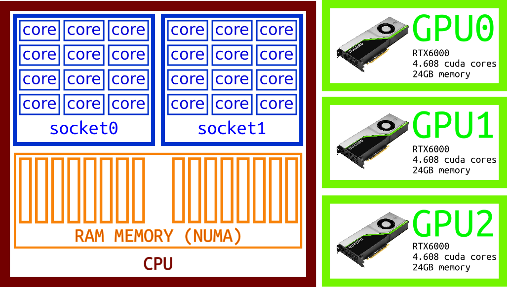
As we did for OpenMP, the same code can be made parallel by adding a few directives.
(example_03.f90)
program converge_pi

   use iso_fortran_env

   implicit none

   integer, parameter :: knd = max(selected_real_kind(15), selected_real_kind(33))
   integer, parameter :: n = huge(1)/1000
   real(kind=knd), parameter :: pi_ref = 3.1415926535897932384626433832795028841971_knd

   integer :: i
   real(kind=knd) :: pi = 0.0, t

   print *, 'KIND      : ', knd
   print *, 'PRECISION : ', precision(pi)
   print *, 'RANGE     : ', range(pi)

   !$ACC PARALLEL LOOP PRIVATE(t) REDUCTION(+:pi)
   do i = 0, n - 1
      t = real(i + 0.5, kind=knd)/n
      pi = pi + 4.0*(1.0/(1.0 + t*t))
   end do
   !$ACC END PARALLEL LOOP

   print *, ""
   print *, "Number of terms in the series : ", n
   print *, "Computed value : ", pi/n
   print *, "Reference vaue : ", pi_ref
   print *, "ABS difference with reference : ", abs(pi_ref - pi/n)

end program converge_pi
The loop is once more surrounded by directives that for this particular case looks very similar to the OpenMP directives presented before.
!$ACC PARALLEL LOOP PRIVATE(t) REDUCTION(+:pi)
do i = 0, n - 1
   t = real(i + 0.5, kind=knd)/n
   pi = pi + 4.0*(1.0/(1.0 + t*t))
end do
!$ACC END PARALLEL LOOP
For the OpenACC version of the code the compilation line is:
$> gfortran -fopenacc example_03.f90
Intel compilers do not support OpenACC The best support comes from NVIDIA compilers
$> nvfortran -acc -Minfo=all example_03.f90
Using directives instead of extending the language offers several advantages:
-
The original source code continues to be valid for those compilers that do know about OpenMP or OpenACC, there is no need to fork the code. If you stay at the level of directives, the code will continue to work without parallelization.
-
The directives provide a very high-level abstraction for parallelism. Other solutions involve deep knowledge about the architecture where the code will run reducing the portability to other systems. Architectures evolve over time and hardware specifics will become a burden for maintainers of the code when it needs to be adapted to newer technologies.
-
The parallelization effort can be done step by step. There is no need to start from scratch planning important rewrites of large portions of the code with will come with more bugs and development costs.
An alternative to OpenMP could be pthreads, and an alternative to OpenACC could be CUDA. Both alternatives suffer from the items mentioned above.
Despite of the similarities at this point, OpenMP and OpenACC were created targeting very different architectures. The idea is that eventually, both will converge into a more general solution. We will now discuss each approach separately, at the end of this discussion we will talk about the efforts to converge both approaches.
Key Points
Use OpenMP for multiple cores, OpenACC and CUDA Fortran for GPUs and MPI for distributed computing.
OpenMP: Parallel Multiprocessing
Overview
Teaching: 60 min
Exercises: 0 minQuestions
How to use the multiple cores on modern computers
Objectives
Learn about programming with OpenMP in Fortran
OpenMP
OpenMP is a directive-based approach to parallelization. OpenMP offers a set of pragmas, ie comments that can be added to the source code to guide the compiler on how it should parallelize certain regions. OpenMP also provides an API, routines, and variables that can be accessed inside the sources and manipulate even further the parallelization.
The first specs for OpenMP date back to 1997. Today most modern Fortran compilers support OpenMP 3.0 and the 3 compilers that we will be using (GNU, Intel, and NVIDIA) support most OpenMP 4.0 or OpenMP 4.5.
OpenMP was created for parallelizing code for shared memory machines. Shared memory machines are those with multiple cores where the cores are able to see, ie address the entire memory of the machine.
Consider now a simple example, one step back from calculating pi and start with a simple print program (hello_omp.f90) to demonstrate how OpenMP works.
program hello

!$OMP PARALLEL

print *, "Hello electron"

!$OMP END PARALLEL

end program hello
Lets compile this code using gfortran
$> gfortran -fopenmp hello_omp.f90 -o hello_omp
Execute the resulting binary:
$> OMP_NUM_THREADS=4 ./hello_omp
Hello electron
Hello electron
Hello electron
Hello electron
To produce a result that is consistent on all machines, we have defined the variable OMP_NUM_THREADS=4 so the code at runtime will create 4 threads regardless of the number of cores on the machine. Not defining this variable and the executable will create by default as many threads as cores it founds on the machine running the code.
In Fortran, the directives !$OMP PARALLEL and !$OMP END PARALLEL will create a block, in this case, a single line block, that will run in parallel. The number of threads that will be created is decided at runtime, at least for this simple parallel block, there is no information about how many threads will be generated.
Notice how two lines of code made this code from running on a single core to running on multiple cores, without any provisions about how many cores it will run. This level of abstraction is one of the big advantages of the approach.
Before OpenMP the alternative for multithreading in Fortran could be something like Pthreads, there is a library for pthreads for IBM AIX machines, the Pthreads Library Module (f_pthread). In this case, we will demonstrate the code in C which is shown below:
#include <pthread.h>
#include <stdio.h>
#include <stdlib.h>
#define PTH_NUM_THREADS 4

void *HelloElectron(void *threadid)
{
	printf("Hello electron\n");
	pthread_exit(NULL);
}

int main (int argc, char *argv[])
{
   pthread_t threads[PTH_NUM_THREADS];
   int rc;
   long t;
   for(t=0; t<PTH_NUM_THREADS; t++){
	rc = pthread_create(&threads[t], NULL, HelloElectron, (void *)t);
   	if (rc) exit(-1);
   }
   pthread_exit(NULL);
   return 0;
}
Notice how this code demands more coding for the same output. The print function is now a function, the creation of each thread is explicit inside a for loop and the number of threads is known during compilation. This last restriction can be removed by adding more extra coding for the allocation of the threads array.
Parallelizing even a simple code will ask for changes to the original structure of the code. That makes the code harder to develop and harder to maintain for those who are not used to multithreading programming. Now the code depends on pthreads even if we change the preprocessor variable to run it serial.
Processes vs threads
OpenMP works by creating threads inside a process and for that reason is important to know the difference between processes and threads. The difference is even more important when we consider MPI where processes potentially running on different machines communicate with each other via exchange of messages.
A process is an instance of a program. Each process has a separate memory address space, which means that a process runs independently and is isolated from other processes. A process cannot directly access shared data in other processes. The kernel of the Operating System manages the execution of all processes, as machines today have multiple cores, that means that at most n processes can be running concurrently on a machine with n cores. As the number of processes is typically larger than the number of cores, each process is receiving CPU time during a certain time interval before the OS switching the core to another process that is demanding attention. Switching from one process to another requires some time (relatively) for saving and loading registers, memory maps, and other resources.
From the other side, a thread is the unit of execution within a process. A process can have just one thread or many threads. Contrary to multiple processes on a machine, each thread in the process shares memory and resources from that process. In single-threaded processes, the process contains one thread. The process and the threads are one and the same, and there is only one thing happening.
What OpenMP does is to create new threads on the same process and as those processes shared resources, they can read and write on the memory addresses assigned to the variables of a process, using this technique multiple threads can effectively complete tasks in parallel when there is data independence in the algorithm being executed.
Many applications today are multithreading, but the way multithreading and in particular OpenMP is used in scientific applications is very different from the multithreading found on desktop applications or games.
For HPC applications, the usual case is for multiple threads to work concurrently on portions of big arrays, reducing values such as sums or products in some cases dividing efforts into separate tasks. The life cycle of threads in OpenMP is more consistent compared for example to multiple threads on a game process. In a game, new threads are generated and destroyed continuously based on the actions of the user.
One of the reasons why parallelization is no a trivial task that can be automatically executed by a compiler by for example adding parallel directives to every loop in a program is due to a non-trivial difficulty to identify data dependencies and data races.
Data dependencies
Consider a DO loop like this:
A(0)=1
DO i=1, 100000
   A(i) = 4*B(i-1) + 3
ENDDO
Assuming that A and B are different arrays, on this loop you can notice that every element of the loop can be computed independent from the others, in fact, there is nothing that forces a given order in the calculation. You can split the loop in 2 or 100 pieces and compute the smaller loops in arbitrary order without affecting the final result. That is very different from:
A(0)=1
DO i=1, 100000
   A(i) = 4*A(i-1) + 3
ENDDO
You can no longer split the loop as computing every element in the loop requires the computation of the value on the previous index.
Sometimes data dependencies can be solved by reordering operations, and separating loops. A data dependency like shown above cannot be eliminated without changing the algorithm itself or this portion of the code serial.
In many cases, there are many loops in a code that do not have data dependencies, some of them worthy of being parallelized.
Consider this simple initialization of an array (simple_omp.f90):
program simple

integer,parameter :: n=huge(1)
integer :: array(n)

print *,n
!$omp parallel do
do i = 1, n
   array(i) = sqrt(real(i))
enddo
!$omp end parallel do

end program
Compile and run this program with and without OpenMP. For example with NVIDIA compilers:
$> nvgfortran -mp -Minfo=all simple_omp.f90
You can notice that running this code on a modern computer could be 5 times faster with OpenMP than without it. The size of the array is one reason, but also the fact that computing the square root of a number takes several CPU cycles to compute. There are many cases with smaller arrays but more complex operations where the lack of data dependencies make those loops good candidates for parallelization.
In this case, there is just one variable inside the loop and the variable array is shared among all the threads that are filling it. In more complex situations there are more variables and we need to decide which variables will be shared and which variables need private copies to prevent a single variable from being overwritten by multiple threads.
Shared and private variables
Consider this example code:
program ratio

   implicit none

   integer, parameter :: n = 40
   real, parameter :: pi = 3.14159265359

   integer :: i, cube_side
   real :: area_to_volume_S(n), area_to_volume_P(n), surface_sphere, volume_cube, diameter

   do i = 1, n
      cube_side = i
      diameter = sqrt(3*real(cube_side)**2)
      surface_sphere = pi*diameter**2
      volume_cube = real(cube_side)**3
      area_to_volume_S(i) = surface_sphere/volume_cube
   end do

!$OMP PARALLEL DO
   do i = 1, n
      cube_side = i
      diameter = sqrt(3*real(cube_side)**2)
      print *, i, cube_side
      surface_sphere = pi*diameter**2
      volume_cube = real(cube_side)**3
      area_to_volume_P(i) = surface_sphere/volume_cube
   end do
!$OMP END PARALLEL DO

   do i = 1, n
      if (abs(area_to_volume_S(i) - area_to_volume_P(i)) > 1e-2) then
         print *, "Wrong value for i=", i, area_to_volume_S(i), area_to_volume_P(i)
      end if
   end do

end program ratio
This code is computing an array area_to_volume that stores the ratio between the surface area of a sphere and the volume of the biggest cube that can be inside the sphere.
The code is doing computing all those values twice.
The same loop is computing area_to_volume_S, the serial version of the loop.
The second loop computes area_to_volume_P and has OpenMP directives which will effectively parallelize the code if the compilation activates those directives.
Except for the print the content of both loops is the same and the content of the arrays should be identical.
Lets compile this code with nvfortran:
$> nvfortran -mp -Minfo=all race-loop_omp.f90 -o race-loop_omp
$> ./race-loop_omp
1             2
9             2
38            2
6             2
11            2
21            2
31            2
34            2
5             2
20            2
26           28
30           28
12           28
23           28
28           28
10           28
18           28
16           28
2            28
33           28
40           28
14           28
3            28
37           28
7            28
39           28
4            28
36           28
17           28
27           28
24           28
29           28
13           28
35           28
25           28
15           28
19           28
32           28
8            28
22           28
Wrong value for i=            1    9.424778        4.712389
Wrong value for i=            2    4.712389       0.3365992
Wrong value for i=            3    3.141593       0.3365992
Wrong value for i=            4    2.356194       0.3365992
Wrong value for i=            5    1.884956        4.712389
Wrong value for i=            6    1.570796        4.712389
Wrong value for i=            7    1.346397       0.3365992
Wrong value for i=            8    1.178097       0.3365992
Wrong value for i=            9    1.047198        4.712389
Wrong value for i=           10   0.9424779       0.3365992
Wrong value for i=           11   0.8567981        4.712389
Wrong value for i=           12   0.7853981       0.3365992
Wrong value for i=           13   0.7249829       0.3365992
Wrong value for i=           14   0.6731984       0.3365992
Wrong value for i=           15   0.6283185       0.3365992
Wrong value for i=           16   0.5890486       0.3365992
Wrong value for i=           17   0.5543987       0.3365992
Wrong value for i=           18   0.5235988       0.3365992
Wrong value for i=           19   0.4960410       0.3365992
Wrong value for i=           20   0.4712389       0.3365992
Wrong value for i=           21   0.4487989        4.712389
Wrong value for i=           22   0.4283990       0.3365992
Wrong value for i=           23   0.4097730       0.3365992
Wrong value for i=           24   0.3926991       0.3365992
Wrong value for i=           25   0.3769911       0.3365992
Wrong value for i=           26   0.3624915       0.3365992
Wrong value for i=           27   0.3490659       0.3365992
Wrong value for i=           29   0.3249924       0.3365992
Wrong value for i=           30   0.3141593       0.3365992
Wrong value for i=           31   0.3040251        4.712389
Wrong value for i=           32   0.2945243       0.3365992
Wrong value for i=           33   0.2855993       0.3365992
Wrong value for i=           34   0.2771994        4.712389
Wrong value for i=           35   0.2692794       0.3365992
Wrong value for i=           36   0.2617994       0.3365992
Wrong value for i=           37   0.2547237       0.3365992
Wrong value for i=           38   0.2480205        4.712389
Wrong value for i=           39   0.2416610       0.3365992
Wrong value for i=           40   0.2356195       0.3365992
Execute multiple times and different discrepancies will appear.
The reason for these errors is that variables such as cube_side, diameter, volume_cube, surface_sphere are all scalars that are shared among all the threads created by OpenMP. One thread can rewrite the value that will be used by another thread evaluating values different from the serial loop.
What we want is to select some values to be private. For that reason there is a clause called private where you can list all the variables that need to be copied on every thread.
The solution is to set the scalars as private. New copies of those variables will be created for each thread created.
!$OMP PARALLEL DO PRIVATE(cube_side, diameter, volume_cube, surface_sphere)
   do i = 1, n
      cube_side = i
      diameter = sqrt(3*real(cube_side)**2)
      print *, i, cube_side
      surface_sphere = pi*diameter**2
      volume_cube = real(cube_side)**3
      area_to_volume_P(i) = surface_sphere/volume_cube
   end do
!$OMP END PARALLEL DO
Data Sharing Attribute Clauses
These Data-sharing attribute clauses apply to parallel blocks.
| clause | Description |
|---|---|
| default(private | firstprivate |shared | none) | Explicitly determines the default data-sharing attributes of variables that are referenced in a parallel, teams, or task generating construct, causing all variables referenced in the construct that have implicitly determined data- sharing attributes to be shared. |
| shared(list) | Declares one or more list items to be shared by tasks generated by a parallel, teams, or task generating construct. The programmer must ensure that storage shared by an explicit task region does not reach the end of its lifetime before the explicit task region completes its execution. |
| private(list) | Declares one or more list items to be private to a task or a SIMD lane. Each task that references a list item that appears in a private clause in any statement in the construct receives a new list item. |
| firstprivate(list) | Declares list items to be private to a task, and initializes each of them with the value that the corresponding original item has when the construct is encountered. |
| lastprivate(list) | Declares one or more list items to be private to an implicit task or to a SIMD lane, and causes the corresponding original list item to be updated after the end of the region. |
These 4 clauses can be better understood with a simple example.
Consider the code below (parallel_clauses_omp.f90)
program clauses

   implicit none
   integer, parameter :: n=10
   integer :: i, a, b, c, d
   character(len=*), parameter :: layout_1 = "(a, 4(a, i12))"
   character(len=*), parameter :: layout_2 = "(a, i4, 4(a, i12))"

   a = 1
   b = 1
   c = 1
   d = 1

   print layout_1, "BEFORE", " SHARED:", a, " PRIVATE:", b, " FIRSTPRIVATE:", c, " LASTPRIVATE:", d

!$OMP PARALLEL DO SHARED(a) PRIVATE(b) FIRSTPRIVATE(c) LASTPRIVATE(d)
   do i = 1, n

      if (n<11) print layout_2, "I=", i, " SHARED:", a, " PRIVATE:", b, " FIRSTPRIVATE:", c, " LASTPRIVATE:", d
      a = a + i
      b = b + i
      c = c + i
      d = d + i
   end do
!$OMP END PARALLEL DO

   print layout_1, "AFTER ", " SHARED:", a, " PRIVATE:", b, " FIRSTPRIVATE:", c, " LASTPRIVATE:", d

end program clauses
We have 4 scalar variables, and we have assigned a value of 1 to each of them.
The loop will increase the value on each iteration.
Notice that the variable a receives all increments but as several threads are reading and writing the variable, race conditions could happen, rare events where one thread reads one value, computes the operation and writes back when another thread have done the same.
Variable b is private, but the value assigned before the loop is lost, each thread receives a new memory location and whatever is on that location will be the initial value.
Variables c and d are also private, but they differ if the initial value inside the loop is initialized or the final value is stored after the loop finishes.
Change the value of n to a very large value, and notice that a produces a different result on each run, those are very rare events so only with a very large loop is possible to trigger them.
For beginners is a good practice to force an explicit declaration of each variable. Use default(none) and you have to decide explicitly if a variable is shared or private.
The default rules in Fortran for sharing are:
Default is shared, except for things that can not possibly be:
- Outer loop index variable
- Inner loop index variables (Fortran)
- Local variables in any called subroutine, unless using save (Fortran).
Consider this example in Fortran:
!$OMP PARALLEL DO
do i=1, n
   do j=1, m
      a(j,i) = b(j,i) + c(j,i)
   end do
end do
!$OMP END PARALLEL DO
The variable i is always private by default,
For OpenMP in Fortran, the variable j is also private but this is not true for OpenMP in C.
It is good to remember that the most optimal way of traversing index on arrays is by operating on adjacent elements in memory. In the case of Fortran, the fast index is the first one, contrary to C where the adjacent elements run on the second index.
Reductions
Private variables die at the end of the thread. We can use lastprivate but the value that is copied to the master thread is only the value for the last iteration in the loop. What if we need to collect somehow the values from all the threads at the end of the loop. Here is where reductions became important.
Consider this example where we are using a series converging to Euler’s number:
program reduction

   implicit none
   integer, parameter :: r15 = selected_real_kind(15)
   integer, parameter :: n = 40
   integer :: i, j

   real(kind=r15) :: euler = 1.0
   real(kind=r15) :: facto
   real(kind=r15), parameter :: e_ref = 2.71828182845904523536028747135266249775724709369995_r15

   !$OMP PARALLEL DO default(none) private(facto) reduction(+:euler)
   do i = 1, n

      facto = real(1)

      ! Not need to run this internal loop in the serial case
      ! Can you remove it and still use OpenMP?
      do j = 1, i
         facto = facto*j
      end do
      euler = euler + real(1)/facto
      print *, "I= ", i, "Euler Number: ", euler, "Error: ", abs(euler - e_ref)

   end do
   !$OMP END PARALLEL DO

   print *, "Final Euler Number: ", euler

end program
We need the variable euler to be private to avoid data races, where the variable is modified inconsistently by threads in the loop.
We also need the variable be initialized with zero as terms of the series will be accumulated there.
Finally, we need the partial sums for euler been added all together to obtain the correct value for the constant.
All that is done by adding reduction(+:euler).
This is a reduction clause that automatically make the variable private, initialize with zero for the child threads and the partial results added with the master thread value for euler=1.0.
Reductions are very important in many cases with loops. These are some reductions available for do loops:
Implicitly Declared Fortran reduction-identifiers
| Identifier | Initializer | Combiner |
|---|---|---|
+ |
omp_priv = 0 | omp_out = omp_in + omp_out |
* |
omp_priv = 1 | omp_out = omp_in * omp_out |
- |
omp_priv = 0 | omp_out = omp_in + omp_out |
.and. |
omp_priv = .true. | omp_out = omp_in .and. omp_out |
.or. |
omp_priv = .false. | omp_out = omp_in .or. omp_out |
.eqv. |
omp_priv = .true. | omp_out = omp_in .eqv. omp_out |
.neqv. |
omp_priv = .false. | omp_out = omp_in .neqv. omp_out |
max |
omp_priv = Least representable number in the reduction list item type | omp_out = max( omp_in, omp_out) |
min |
omp_priv = Largest representable number in the reduction list item type | omp_out = min( omp_in, omp_out) |
iand |
omp_priv = All bits on | omp_out = iand( omp_in, omp_out) |
ior |
omp_priv = 0 | omp_out = ior( omp_in, omp_out) |
ieor |
omp_priv = 0 | omp_out = ieor( omp_in, omp_out) |
A more general Parallel construct
So far we have been using !$OMP PARALLEL DO.
This is a convenient construct for parallelizing DO loops in fortran.
OpenMP offers a more general construct !$OMP PARALLEL that ask the system to span a number of threads and leave how those therads are used to other constructs that can use those threads.
Barrier and Critical directives
OpenMP has a variety of tools for managing processes. One of the more prominent forms of control comes with the barrier:
!$OMP BARRIER
…and the critical directives:
!$OMP CRITICAL
...
!$OMP END CRITICAL
The barrier directive stops all processes from proceeding to the next line of code until all processes have reached the barrier. This allows a programmer to synchronize processes in the parallel program.
A critical directive ensures that a line of code is only run by one process at a time, ensuring thread safety in the body of code.
One simple example consists on ensuring that the messages from different threads print in order
program main

use omp_lib

implicit none

integer :: i, thread_id

!$OMP PARALLEL PRIVATE(thread_id)
    thread_id = OMP_GET_THREAD_NUM()

    do i=0, OMP_GET_MAX_THREADS()
        if (i == thread_id) then
            print *, "Hello OpenMP from thread: ", thread_id
        end if
        !$OMP BARRIER
    end do
!$OMP END PARALLEL

stop

end program
A thread-safe section of the code can be done by declaring the block CRITICAL. In this case we are computing function sinc(pi*z) where we set z=1/4
program main

   use omp_lib

   implicit none

   integer, parameter :: k15 = selected_real_kind(15)
   real(kind=k15) :: partial_prod, total_prod
   integer :: i
   real(kind=k15)    :: z=0.25

!$OMP PARALLEL PRIVATE(partial_prod) SHARED(total_prod)
   partial_prod = 1;
   total_prod = 1;
   !$OMP DO
   do i = 1, huge(i)
      partial_prod = partial_prod * (1.0 - z**2 / real(i)**2)
   end do
   !$OMP END DO

   !$OMP CRITICAL
   total_prod = total_prod * partial_prod
   !$OMP END CRITICAL

!$OMP END PARALLEL
   print *, "Total Prod: ", total_prod

end program
Multitasks
module thetables

   integer, parameter :: i6 = selected_int_kind(6)
   integer, parameter :: r9 = selected_real_kind(9)

contains

   subroutine prime_table(prime_num, primes)

      implicit none

      integer(kind=i6) prime_num

      integer(kind=i6) i
      integer(kind=i6) j
      integer(kind=i6) p
      logical prime
      integer(kind=i6) primes(prime_num)

      i = 2
      p = 0

      do while (p < prime_num)

         prime = .true.

         do j = 2, i - 1
            if (mod(i, j) == 0) then
               prime = .false.
               exit
            end if
         end do

         if (prime) then
            p = p + 1
            primes(p) = i
         end if

         i = i + 1

      end do

      return
   end

   subroutine sine_table(sine_num, sines)

      implicit none

      integer(kind=i6) sine_num

      real(kind=r9) a
      integer(kind=i6) i
      integer(kind=i6) j
      real(kind=r9), parameter :: r8_pi = 3.141592653589793D+00
      real(kind=r9) sines(sine_num)

      do i = 1, sine_num
         sines(i) = 0.0D+00
         do j = 1, i
            a = real(j - 1, kind=r9)*r8_pi/real(sine_num - 1, kind=r9)
            sines(i) = sines(i) + sin(a)
         end do
      end do

      return
   end

   subroutine cosine_table(cosine_num, cosines)

      implicit none

      integer(kind=i6) cosine_num

      real(kind=r9) a
      integer(kind=i6) i
      integer(kind=i6) j
      real(kind=r9), parameter :: r8_pi = 3.141592653589793D+00
      real(kind=r9) cosines(cosine_num)

      do i = 1, cosine_num
         cosines(i) = 0.0D+00
         do j = 1, i
            a = real(j - 1, kind=r9)*r8_pi/real(cosine_num - 1, kind=r9)
            cosines(i) = cosines(i) + sin(a)
         end do
      end do

      return
   end

end module thetables

program main

   use omp_lib
   use thetables

   implicit none

   integer(kind=i6) prime_num
   integer(kind=i6), allocatable :: primes(:)
   integer(kind=i6) sine_num, cosine_num
   real(kind=r9), allocatable :: sines(:), cosines(:)
   real(kind=r9) wtime
   real(kind=r9) wtime1, wtime2, wtime3


   write (*, '(a)') ' '
   write (*, '(a)') 'MULTITASK_OPENMP:'
   write (*, '(a)') '  FORTRAN90/OpenMP version'
   write (*, '(a)') '  Demonstrate how OpenMP can "multitask" by using the'
   write (*, '(a)') &
      '  SECTIONS directive to carry out several tasks in parallel.'

   prime_num = 20000
   allocate (primes(1:prime_num))
   sine_num = 20000
   cosine_num = 40000
   allocate (sines(1:sine_num))
   allocate (cosines(1:cosine_num))

   wtime = omp_get_wtime()

!$omp parallel shared ( prime_num, primes, sine_num, sines )

   !$omp sections

   !$omp section
   wtime1 = omp_get_wtime()
   call prime_table(prime_num, primes)
   wtime1 = omp_get_wtime() - wtime1
   !$omp section
   wtime2 = omp_get_wtime()
   call sine_table(sine_num, sines)
   wtime2 = omp_get_wtime() - wtime2
   !$omp section
   wtime3 = omp_get_wtime()
   call cosine_table(cosine_num, cosines)
   wtime3 = omp_get_wtime() - wtime3
   !$omp end sections

!$omp end parallel

   wtime = omp_get_wtime() - wtime

   write (*, '(a)') ' '
   write (*, '(a,i6)') '  Number of primes computed was ', prime_num
   write (*, '(a,i12)') '  Last prime was ', primes(prime_num)
   write (*, '(a,i6)') '  Number of sines computed was ', sine_num
   write (*, '(a,g14.6)') '  Last sine computed was ', sines(sine_num)
   write (*, '(a,i6)') '  Number of cosines computed was ', cosine_num
   write (*, '(a,g14.6)') '  Last cosine computed was ', cosines(cosine_num)
   write (*, '(a)') ' '
   write (*, '(a,g14.6)') '  Elapsed time = ', wtime
   write (*, '(a,g14.6)') '  Task 1 time = ', wtime1
   write (*, '(a,g14.6)') '  Task 2 time = ', wtime2
   write (*, '(a,g14.6)') '  Task 3 time = ', wtime3
!
!  Free memory.
!
   deallocate (primes)
   deallocate (sines)
   deallocate (cosines)
!
!  Terminate.
!
   write (*, '(a)') ' '
   write (*, '(a)') 'MULTITASK_OPENMP:'
   write (*, '(a)') '  Normal end of execution.'
   write (*, '(a)') ' '

   stop
end
Key Points
OpenMP is a directive-based approach for parallelization.
Exercises
Overview
Teaching: 0 min
Exercises: 60 minQuestions
Objectives
Exercise 1:
Write a Fortran program that writes “Hello OpenMP”. Compile and execute.
Convert the previous Fortran program in multithreaded with a
paralelldirectiveLoad the omp_lib module and print also the thread number using the function
omp_get_thread_num()andomp_get_num_threads()Store the values for the number of threads and thread ID on variables before printing
What is the difference bettween making those variables public or private.
Exercise 2:
Write a Fortran code that computes the integral of a function f(x)=log(pix)sin(pi*x)**2 + x in the range [1,10]
Use rectangles to approximate the integral and use an OpenMP parallel loop. (*) An alternative could be using trapezoids instead of triangles.
Compare the performance of the serial code compared with the parallel version.
Use the function omp_get_wtime() to get the time spent on the loop. The function returns a real and can be used before and after the loop.
Exercise 3:
Use the following product to approximate pi
Use the reduction for a product to an approximation of pi
How many terms are needed to get 4 good digits?
Key Points
Adjurn
Overview
Teaching: min
Exercises: minQuestions
Objectives
Use the break layout for placeholder episodes representing coffee breaks and lunches.
These episodes do not have exercises, questions, objectives, or keypoints in their metadata,
but must have a “break” field to show how long the break is (in minutes).
Key Points
OpenACC: Parallel Accelerators
Overview
Teaching: 60 min
Exercises: 0 minQuestions
How to write code for GPUs from a directive-base model?
OpenACC
OpenACC is another directive-based model for parallel programming. It is similar to OpenMP but focused more on Accelerators rather than Multicore processors as OpenMP.
Similar to OpenMP, the idea is to take the original code and introduce directives in places that could benefit from parallel programming. If you use only directives, the code still compiles with compilers that do not support OpenACC and the code will run serially as usual.
OpenACC is another directive-based approach for parallel programming with a more general scope than the original OpenMP. Before version 4.0, OpenMP was designed to provide parallelism to multicore systems, an alternative to more tedious alternatives like programming with pthreads. With the advent of accelerators, like GPUs, a more general paradigm was needed that preserve the nice features that OpenMP bring to parallel computing.
An accelerator is, in general, a device that is able to perform certain classes of computations with more performance than the CPU. Accelerators such as GPUs come with a high bandwidth memory that is separated from the main CPU RAM. Any processing that happens in an accelerator must first transfer the data from the CPU memory into the device memory and at the end of the calculation, move the data back.
Currently, the best support for OpenACC comes from NVIDIA compilers (nvfortran), followed by GCC compilers (gfortran). Intel compilers do not support OpenACC and there is no plan for support it in the near future.
In this lesson, we will follow a similar path as we did for OpenMP. First, we parallelize a loop and later we generalize the operation to more abstract parallel entities, such as tasks. Most of the complexity added to OpenACC compared to OpenMP comes from the fact that accelerators usually work on their own memory space, meaning that to use them, data must be transferred into the accelerator and final data move it back to CPU memory. That is more complex than the way OpenMP works where data is always in CPU memory and threads are able to see that memory space directly and operate with it.
The structure of OpenACC directives in Fortran is as follows:
!$acc <directive> [clause, [[,] clause] . . . ]
This is called and OpenACC construct. A construct is made of one directive followed by one or more clauses
If directive and its clauses became too long, you can split the line using backslash(\) at the end of the line to extend the interpretation to the next line.
Beyond using OpenACC directives you could prefer to have fine detail on the parallel execution. OpenACC offers an API similar to OpenMP which also offers one. Using them and the code will only be able to work with the OpenACC runtime environment.
In Fortran, the API is activated by including the module openacc
use openacc
First steps with OpenACC
Consider this small code (example_01.f90):
module process_mod
contains
   subroutine process(a, b, n)
      real :: a(:), b(:)
      integer :: n, i

      print *, "subroutine process..."
!$ACC PARALLEL LOOP
      do i = 1, n
         b(i) = exp(sin(a(i)))
      end do
!$ACC END PARALLEL LOOP
   end subroutine
end module process_mod

program simple

   use process_mod

   integer, parameter :: n = 1*10**9
   integer :: i
   real, allocatable:: a(:), b(:)
   allocate (a(n), b(n))

   print *, "initializing array..."
!$ACC PARALLEL LOOP
   do i = 1, n
      a(i) = asin(log(real(i)))
   end do
!ACC END PARALLEL LOOP

   call process(a, b, n)

end program simple
This code captures the essence of many scientific code. It has a subroutine inside a module and there is a loop to initialize an array and another loop to produce a computation.
On these two loops we enclose them with OpenACC directives. Before we discuss those lets first compile the code and run it under several conditions. For OpenACC we will use the NVIDIA Compilers (Formerly PGI compilers). As we will execute the code on a GPU the first step is to request an interactive session on a compute node with GPU. Execute this command to request 1 node, 8 cores and 1 GPU for 4 hours
$> qsub -I -q comm_gpu_inter -l nodes=1:ppn=8:gpus=1
The command above request 1 GPU card, 8 CPU cores on 1 node.
The default wall time for comm_gpu_inter queue is 4 hours, so that is the amount of time that is given when the job start running.
The reason for selecting 8 hours is that most GPU compute nodes offer 3 GPU cards and those machines have 24 cores, the ratio then is 8 CPU cores for each GPU card.
There are ways of using more than one GPU card but 1 GPU is enough during these examples and exercises.
The job will run on a GPU node.
You can check the presence of the GPU by running the command nvidia-smi.
The output is shown below:
Wed Aug 03 12:37:57 2021
+-----------------------------------------------------------------------------+
| NVIDIA-SMI 465.19.01    Driver Version: 465.19.01    CUDA Version: 11.3     |
|-------------------------------+----------------------+----------------------+
| GPU  Name        Persistence-M| Bus-Id        Disp.A | Volatile Uncorr. ECC |
| Fan  Temp  Perf  Pwr:Usage/Cap|         Memory-Usage | GPU-Util  Compute M. |
|                               |                      |               MIG M. |
|===============================+======================+======================|
|   0  NVIDIA Quadro P...  Off  | 00000000:AF:00.0 Off |                  Off |
| 26%   19C    P8     8W / 250W |      0MiB / 24449MiB |      0%   E. Process |
|                               |                      |                  N/A |
+-------------------------------+----------------------+----------------------+

+-----------------------------------------------------------------------------+
| Processes:                                                                  |
|  GPU   GI   CI        PID   Type   Process name                  GPU Memory |
|        ID   ID                                                   Usage      |
|=============================================================================|
|  No running processes found                                                 |
+-----------------------------------------------------------------------------+
Once you get assigned one of the GPU compute nodes. You need to load the module for the NVIDIA HPC SDK and change to the folder with the code examples:
$> module load lang/nvidia/nvhpc
$> cd Modern-Fortran/files/openacc
The NVIDIA compilers offer some environment variables that can be used for performance analysis during executions. Execute this to enable the timing when running with OpenACC on GPUs:
$> export PGI_ACC_TIME=1
For our first compilation, we will compile without any special argument for the compiler. By default, the compiler will ignore entirely any OpenACC directive and compile a pure Fortran code.
$> nvfortran example_01.f90
$> time ./a.out
initializing array...
subroutine process...

real	0m27.616s
user	0m26.072s
sys	  0m1.479s
We are using time to get the amount of time took by the execution of the code.
Notice that there are 2 loops that take most of the time, one initializing the array a and a second that computes b.
We have used a few functions like exp, sin and their inverses.
Those are simple mathematical operations but computing with them takes a few CPU cycles for each value, making them particularly expensive for a large array like a.
Compiling the code like above, the resulting executable will only run on one core.
The timing says that 27 seconds are needed on the machine.
Example 1: SAXPY
For our first example we will demonstrate the use of OpenACC to parallelize the function Y = aX + Y,
module mod_saxpy

contains

   subroutine saxpy(n, a, x, y)

      implicit none

      real :: x(:), y(:), a
      integer :: n, i

!$ACC PARALLEL LOOP
      do i = 1, n
         y(i) = a*x(i) + y(i)
      end do
!$ACC END PARALLEL LOOP

   end subroutine saxpy

end module mod_saxpy

program main

   use mod_saxpy

   implicit none

   integer, parameter :: n = huge(n)
   real :: x(n), y(n), a = 2.3
   integer :: i

   print *, "Initializing X and Y..."

!$ACC PARALLEL LOOP
   do i = 1, n
      x(i) = sqrt(real(i))
      y(i) = sqrt(1.0/real(i))
   end do
!$ACC END PARALLEL LOOP

   print *, "Computing the SAXPY operation..."

!$ACC PARALLEL LOOP
   do i = 1, n
      y(i) = a*x(i) + y(i)
   end do
!$ACC END PARALLEL LOOP

   call saxpy(n, a, x, y)

end program main
There are two sections parallelized in the code, on each one of them there is some data being implicitly moved to the GPU memory an back to CPU memory.
Laplace example
This is a good example for demonstrating how a code can be improved step by step adding OpenACC directives. We start with the serial version of the code.
Serial Laplace
program serial
      implicit none

      !Size of plate
      integer, parameter             :: columns=1000
      integer, parameter             :: rows=1000
      double precision, parameter    :: max_temp_error=0.01

      integer                        :: i, j, max_iterations, iteration=1
      double precision               :: dt=100.0
      real                           :: start_time, stop_time

      double precision, dimension(0:rows+1,0:columns+1) :: temperature, temperature_last

      print*, 'Maximum iterations [100-4000]?'
      read*,   max_iterations

      call cpu_time(start_time)      !Fortran timer

      call initialize(temperature_last)

      !do until error is minimal or until maximum steps
      do while ( dt > max_temp_error .and. iteration <= max_iterations)

         do j=1,columns
            do i=1,rows
               temperature(i,j)=0.25*(temperature_last(i+1,j)+temperature_last(i-1,j)+ &
                                      temperature_last(i,j+1)+temperature_last(i,j-1) )
            enddo
         enddo

         dt=0.0

         !copy grid to old grid for next iteration and find max change
         do j=1,columns
            do i=1,rows
               dt = max( abs(temperature(i,j) - temperature_last(i,j)), dt )
               temperature_last(i,j) = temperature(i,j)
            enddo
         enddo

         !periodically print test values
         if( mod(iteration,100).eq.0 ) then
            call track_progress(temperature, iteration)
         endif

         iteration = iteration+1

      enddo

      call cpu_time(stop_time)

      print*, 'Max error at iteration ', iteration-1, ' was ',dt
      print*, 'Total time was ',stop_time-start_time, ' seconds.'

end program serial


! initialize plate and boundery conditions
! temp_last is used to to start first iteration
subroutine initialize( temperature_last )
      implicit none

      integer, parameter             :: columns=1000
      integer, parameter             :: rows=1000
      integer                        :: i,j

      double precision, dimension(0:rows+1,0:columns+1) :: temperature_last

      temperature_last = 0.0

      !these boundary conditions never change throughout run

      !set left side to 0 and right to linear increase
      do i=0,rows+1
         temperature_last(i,0) = 0.0
         temperature_last(i,columns+1) = (100.0/rows) * i
      enddo

      !set top to 0 and bottom to linear increase
      do j=0,columns+1
         temperature_last(0,j) = 0.0
         temperature_last(rows+1,j) = ((100.0)/columns) * j
      enddo

end subroutine initialize


!print diagonal in bottom corner where most action is
subroutine track_progress(temperature, iteration)
      implicit none

      integer, parameter             :: columns=1000
      integer, parameter             :: rows=1000
      integer                        :: i,iteration

      double precision, dimension(0:rows+1,0:columns+1) :: temperature

      print *, '---------- Iteration number: ', iteration, ' ---------------'
      do i=5,0,-1
         write (*,'("("i4,",",i4,"):",f6.2,"  ")',advance='no') &
                   rows-i,columns-i,temperature(rows-i,columns-i)
      enddo
      print *
end subroutine track_progress
Bad OpenACC Laplace
program serial
      implicit none

      !Size of plate
      integer, parameter             :: columns=1000
      integer, parameter             :: rows=1000
      double precision, parameter    :: max_temp_error=0.01

      integer                        :: i, j, max_iterations, iteration=1
      double precision               :: dt=100.0
      real                           :: start_time, stop_time

      double precision, dimension(0:rows+1,0:columns+1) :: temperature, temperature_last

      print*, 'Maximum iterations [100-4000]?'
      read*,   max_iterations

      call cpu_time(start_time)      !Fortran timer

      call initialize(temperature_last)

      !do until error is minimal or until maximum steps
      do while ( dt > max_temp_error .and. iteration <= max_iterations)

         !$acc kernels
         do j=1,columns
            do i=1,rows
               temperature(i,j)=0.25*(temperature_last(i+1,j)+temperature_last(i-1,j)+ &
                                      temperature_last(i,j+1)+temperature_last(i,j-1) )
            enddo
         enddo
         !$acc end kernels

         dt=0.0

         !copy grid to old grid for next iteration and find max change
         !$acc kernels
         do j=1,columns
            do i=1,rows
               dt = max( abs(temperature(i,j) - temperature_last(i,j)), dt )
               temperature_last(i,j) = temperature(i,j)
            enddo
         enddo
         !$acc end kernels

         !periodically print test values
         if( mod(iteration,100).eq.0 ) then
            call track_progress(temperature, iteration)
         endif

         iteration = iteration+1

      enddo

      call cpu_time(stop_time)

      print*, 'Max error at iteration ', iteration-1, ' was ',dt
      print*, 'Total time was ',stop_time-start_time, ' seconds.'

end program serial


! initialize plate and boundery conditions
! temp_last is used to to start first iteration
subroutine initialize( temperature_last )
      implicit none

      integer, parameter             :: columns=1000
      integer, parameter             :: rows=1000
      integer                        :: i,j

      double precision, dimension(0:rows+1,0:columns+1) :: temperature_last

      temperature_last = 0.0

      !these boundary conditions never change throughout run

      !set left side to 0 and right to linear increase
      do i=0,rows+1
         temperature_last(i,0) = 0.0
         temperature_last(i,columns+1) = (100.0/rows) * i
      enddo

      !set top to 0 and bottom to linear increase
      do j=0,columns+1
         temperature_last(0,j) = 0.0
         temperature_last(rows+1,j) = ((100.0)/columns) * j
      enddo

end subroutine initialize


!print diagonal in bottom corner where most action is
subroutine track_progress(temperature, iteration)
      implicit none

      integer, parameter             :: columns=1000
      integer, parameter             :: rows=1000
      integer                        :: i,iteration

      double precision, dimension(0:rows+1,0:columns+1) :: temperature

      print *, '---------- Iteration number: ', iteration, ' ---------------'
      do i=5,0,-1
         write (*,'("("i4,",",i4,"):",f6.2,"  ")',advance='no') &
                   rows-i,columns-i,temperature(rows-i,columns-i)
      enddo
      print *
end subroutine track_progress
Efficient OpenACC Laplace
program serial
      implicit none

      !Size of plate
      integer, parameter             :: columns=1000
      integer, parameter             :: rows=1000
      double precision, parameter    :: max_temp_error=0.01

      integer                        :: i, j, max_iterations, iteration=1
      double precision               :: dt=100.0
      real                           :: start_time, stop_time

      double precision, dimension(0:rows+1,0:columns+1) :: temperature, temperature_last

      print*, 'Maximum iterations [100-4000]?'
      read*,   max_iterations

      call cpu_time(start_time)      !Fortran timer

      call initialize(temperature_last)

      !do until error is minimal or until maximum steps
      !$acc data copy(temperature_last), create(temperature)
      do while ( dt > max_temp_error .and. iteration <= max_iterations)

         !$acc kernels
         do j=1,columns
            do i=1,rows
               temperature(i,j)=0.25*(temperature_last(i+1,j)+temperature_last(i-1,j)+ &
                                      temperature_last(i,j+1)+temperature_last(i,j-1) )
            enddo
         enddo
         !$acc end kernels

         dt=0.0

         !copy grid to old grid for next iteration and find max change
         !$acc kernels
         do j=1,columns
            do i=1,rows
               dt = max( abs(temperature(i,j) - temperature_last(i,j)), dt )
               temperature_last(i,j) = temperature(i,j)
            enddo
         enddo
         !$acc end kernels

         !periodically print test values
         if( mod(iteration,100).eq.0 ) then
            call track_progress(temperature, iteration)
         endif

         iteration = iteration+1

      enddo
      !$acc end data

      call cpu_time(stop_time)

      print*, 'Max error at iteration ', iteration-1, ' was ',dt
      print*, 'Total time was ',stop_time-start_time, ' seconds.'

end program serial


! initialize plate and boundery conditions
! temp_last is used to to start first iteration
subroutine initialize( temperature_last )
      implicit none

      integer, parameter             :: columns=1000
      integer, parameter             :: rows=1000
      integer                        :: i,j

      double precision, dimension(0:rows+1,0:columns+1) :: temperature_last

      temperature_last = 0.0

      !these boundary conditions never change throughout run

      !set left side to 0 and right to linear increase
      do i=0,rows+1
         temperature_last(i,0) = 0.0
         temperature_last(i,columns+1) = (100.0/rows) * i
      enddo

      !set top to 0 and bottom to linear increase
      do j=0,columns+1
         temperature_last(0,j) = 0.0
         temperature_last(rows+1,j) = ((100.0)/columns) * j
      enddo

end subroutine initialize


!print diagonal in bottom corner where most action is
subroutine track_progress(temperature, iteration)
      implicit none

      integer, parameter             :: columns=1000
      integer, parameter             :: rows=1000
      integer                        :: i,iteration

      double precision, dimension(0:rows+1,0:columns+1) :: temperature

      print *, '---------- Iteration number: ', iteration, ' ---------------'
      do i=5,0,-1
         write (*,'("("i4,",",i4,"):",f6.2,"  ")',advance='no') &
                   rows-i,columns-i,temperature(rows-i,columns-i)
      enddo
      print *
end subroutine track_progress
Updating Temperature
program serial
      implicit none

      !Size of plate
      integer, parameter             :: columns=1000
      integer, parameter             :: rows=1000
      double precision, parameter    :: max_temp_error=0.01

      integer                        :: i, j, max_iterations, iteration=1
      double precision               :: dt=100.0
      real                           :: start_time, stop_time

      double precision, dimension(0:rows+1,0:columns+1) :: temperature, temperature_last

      print*, 'Maximum iterations [100-4000]?'
      read*,   max_iterations

      call cpu_time(start_time)      !Fortran timer

      call initialize(temperature_last)

      !do until error is minimal or until maximum steps
      !$acc data copy(temperature_last), create(temperature)
      do while ( dt > max_temp_error .and. iteration <= max_iterations)

         !$acc kernels
         do j=1,columns
            do i=1,rows
               temperature(i,j)=0.25*(temperature_last(i+1,j)+temperature_last(i-1,j)+ &
                                      temperature_last(i,j+1)+temperature_last(i,j-1) )
            enddo
         enddo
         !$acc end kernels

         dt=0.0

         !copy grid to old grid for next iteration and find max change
         !$acc kernels
         do j=1,columns
            do i=1,rows
               dt = max( abs(temperature(i,j) - temperature_last(i,j)), dt )
               temperature_last(i,j) = temperature(i,j)
            enddo
         enddo
         !$acc end kernels

         !periodically print test values
         if( mod(iteration,100).eq.0 ) then
            !$acc update host(temperature)
            call track_progress(temperature, iteration)
         endif

         iteration = iteration+1

      enddo
      !$acc end data

      call cpu_time(stop_time)

      print*, 'Max error at iteration ', iteration-1, ' was ',dt
      print*, 'Total time was ',stop_time-start_time, ' seconds.'

end program serial


! initialize plate and boundery conditions
! temp_last is used to to start first iteration
subroutine initialize( temperature_last )
      implicit none

      integer, parameter             :: columns=1000
      integer, parameter             :: rows=1000
      integer                        :: i,j

      double precision, dimension(0:rows+1,0:columns+1) :: temperature_last

      temperature_last = 0.0

      !these boundary conditions never change throughout run

      !set left side to 0 and right to linear increase
      do i=0,rows+1
         temperature_last(i,0) = 0.0
         temperature_last(i,columns+1) = (100.0/rows) * i
      enddo

      !set top to 0 and bottom to linear increase
      do j=0,columns+1
         temperature_last(0,j) = 0.0
         temperature_last(rows+1,j) = ((100.0)/columns) * j
      enddo

end subroutine initialize


!print diagonal in bottom corner where most action is
subroutine track_progress(temperature, iteration)
      implicit none

      integer, parameter             :: columns=1000
      integer, parameter             :: rows=1000
      integer                        :: i,iteration

      double precision, dimension(0:rows+1,0:columns+1) :: temperature

      print *, '---------- Iteration number: ', iteration, ' ---------------'
      do i=5,0,-1
         write (*,'("("i4,",",i4,"):",f6.2,"  ")',advance='no') &
                   rows-i,columns-i,temperature(rows-i,columns-i)
      enddo
      print *
end subroutine track_progress
Key Points
OpenACC is another directive-base model for parallel programming.
OpenACC is similar to OpenMP but take advantage of accelerators such as GPUs
CUDA Fortran
Overview
Teaching: 60 min
Exercises: 0 minQuestions
How to program in CUDA Fortran?
Objectives
Learn about the CUDA Fortran interface
CUDA Fortran
Graphic processing units or GPUs have evolved into programmable, highly parallel computational units with very high memory bandwidth, and potential for scientific applications. GPU designs are optimized for the kind of computations found in graphics rendering, but are general enough to be useful in many cases involving data-parallelism, linear algebra, and other common use cases in scientific computing.
CUDA Fortran is the Fortran interface to the CUDA parallel computing platform.
If you are familiar with CUDA C, then you are already well on your way to using
CUDA Fortran is based on the CUDA C runtime API.
There are a few differences in how CUDA concepts are expressed using
Fortran 90 constructs, but the programming model for both CUDA Fortran and
CUDA C is the same.
CUDA Fortran is essentially Fortran with a few extensions that allow one to execute subroutines on the GPU by many threads in parallel.
CUDA Programming Model Basics
Before we jump into CUDA Fortran code, those new to CUDA will benefit from a basic description of the CUDA programming model and some of the terminology used.
The CUDA programming model is a heterogeneous model in which both the CPU and GPU are used. In CUDA, the host refers to the CPU and its memory, while the device refers to the GPU and its memory. Code running on the host manages the memory on both the host and device and also launches kernels which are subroutines executed on the device. These kernels are executed by many GPU threads in parallel.
Given the heterogeneous nature of the CUDA programming model, a typical sequence of operations for a CUDA Fortran code is:
- Declare and allocate a host and device memory.
- Initialize host data.
- Transfer data from the host to the device.
- Execute one or more kernels.
- Transfer results from the device to the host.
Keeping this sequence of operations in mind, let’s look at a CUDA Fortran example.
A First CUDA Fortran Program
SAXPY stands for “Single-precision A*X Plus Y”, and is a good “hello world” example for parallel computation. In this post I want to dissect a similar version of SAXPY, explaining in detail what is done and why. The complete SAXPY code is:
module mathOps
contains
  attributes(global) subroutine saxpy(x, y, a)
    implicit none
    real :: x(:), y(:)
    real, value :: a
    integer :: i, n
    n = size(x)
    i = blockDim%x * (blockIdx%x - 1) + threadIdx%x
    if (i <= n) y(i) = y(i) + a*x(i)
  end subroutine saxpy
end module mathOps

program testSaxpy
  use mathOps
  use cudafor
  implicit none
  integer, parameter :: N = 1024000
  real :: x(N), y(N), a
  real, device :: x_d(N), y_d(N)
  type(dim3) :: grid, tBlock

  tBlock = dim3(256,1,1)
  grid = dim3(ceiling(real(N)/tBlock%x),1,1)

  call random_number(x)
  call random_number(y)
  call random_number(a)

  !x = 1.0; y = 2.0; a = 2.0
  x_d = x
  y_d = y
  call saxpy<<<grid, tBlock>>>(x_d, y_d, a)
  y = y_d

  print *, "Size of arrays: ", N
  print *, 'Grid             : ', grid
  print *, 'Threads per block: ', tBlock

  print *, "Constant a:", a
  print *, 'Average values ', sum(abs(x))/N, sum(abs(y))/N
end program testSaxpy
The module mathOps above contains the subroutine saxpy, which is the kernel that is performed on the GPU, and the program testSaxpy is the host code. Let’s begin our discussion of this program with the host code.
Host Code
The program testSaxpy uses two modules:
  use mathOps
  use cudafor
The first is the user-defined module mathOps which contains the saxpy kernel, and the second is the cudafor module which contains the CUDA Fortran definitions. In the variable declaration section of the code, two sets of arrays are defined:
  real :: x(N), y(N), a
  real, device :: x_d(N), y_d(N)
The real arrays x and y are the host arrays, declared in the typical
fashion, and the x_d and y_d arrays are device arrays declared with
the device variable attribute. As with CUDA C, the host and device in CUDA
Fortran have separate memory spaces, both of which are managed from host code.
But while CUDA C declares variables that reside in device memory in a
conventional manner and uses CUDA-specific routines to allocate data on
the GPU and transfer data between the CPU and GPU, CUDA Fortran uses the
device variable attribute to indicate which data reside in device memory
and uses conventional means to allocate and transfer data. The arrays
x_d and y_d could have been declared with the allocatable in addition
to the device attribute and allocated with the F90 allocate statement.
One consequence of the strong typing in Fortran coupled with the presence of the device attribute is that transfers between the host and device can be performed simply by assignment statements. The host-to-device transfers prior to the kernel launch are done by:
  x_d = x
  y_d = y
while the device-to-host transfer of the result is done by:
y = y_d
The saxpy kernel is launched by the statement:
call saxpy<<<grid,tBlock>>>(x_d, y_d, a)
The information between the triple chevrons is the execution configuration, which dictates how many device threads execute the kernel in parallel. In CUDA there is a hierarchy of threads in software which mimics how thread processors are grouped on the GPU. In CUDA we speak of launching a kernel with a grid of thread blocks. The second argument in the execution configuration specifies the number of threads in a thread block, and the first specifies the number of thread blocks in the grid. Threads in a thread block can be arranged in a multidimensional manner to accommodate the multidimensional nature of the underlying problem, and likewise thread blocks can be arranged as such in a grid. It is for this reason that the derived type dim3, which contains x, y, and z components, is used for these two execution configuration parameters. In a one-dimensional case such as this, these two execution configuration parameters could also have been specified as integers. In this case we launch the kernel with thread blocks containing 256 threads, and use the ceiling function to determine the number of thread blocks required to process all N elements of the arrays:
  tBlock = dim3(256,1,1)
  grid = dim3(ceiling(real(N)/tBlock%x),1,1)
For cases where the number of elements in the arrays is not evenly divisible by the thread block size, the kernel code must check for out-of-bounds memory accesses.
Device Code
We now move on to the kernel code, which once again is:
  attributes(global) subroutine saxpy(x, y, a)
    implicit none
    real :: x(:), y(:)
    real, value :: a
    integer :: i, n
    n = size(x)
    i = blockDim%x * (blockIdx%x - 1) + threadIdx%x
    if (i <= n) y(i) = y(i) + a*x(i)
  end subroutine saxpy
The saxpy kernel is differentiated from host subroutines via the
attributes(global) qualifier.
In the variable declarations, the device attribute is not needed as it is
assumed that in device code all arguments reside on the device.
This is the case for the first two arguments of this kernel, which
correspond to the device arrays x_d and y_d in host code. However, the
last argument, the parameter a, was not transferred to the device in
host code. Because Fortran passes arguments by reference rather than
value, accessing a host variable from the device would cause an error
unless the value variable attribute is used in such cases, which instructs
the compiler to pass such arguments by value.
After the variable declarations, there are only three lines in our saxpy kernel.
As mentioned earlier, the kernel is executed by multiple threads in parallel.
If we want each thread to process an element of the resultant array, then we
need a means of distinguishing and identifying each thread. This is
accomplished through the predefined variables blockDim, blockIdx, and
threadIdx. These predefined variables are of type dim3, and are analogous to
the execution configuration parameters in host code. The predefined variable
blockDim in the kernel is equivalent to the thread block specified in host
code by the second execution configuration parameter.
The predefined variables threadIdx and blockIdx give the identity of the
thread within the thread block and the thread block within the grid,
respectively. The expression:
i = blockDim%x * (blockIdx%x - 1) + threadIdx%x
generates a global index that is used to access elements of the arrays. Note that in CUDA Fortran, the components of threadIdx and blockIdx have unit offset, so the first thread in a block has threadIdx%x=1 and the first block in the grid has blockIdx%x=1. This differs from CUDA C which has zero offset for these built-in variables, where the equivalent expression for an index used to access C arrays would be:
i = blockDim.x*blockIdx.x + threadIdx.x;
Before this index is used to access array elements, its value is checked against the number of elements, obtained from the size() intrinsic, to ensure there are no out-of-bounds memory accesses. This check is required for cases where the number of elements in an array is not evenly divisible by the thread block size, and as a result the number of threads launched by the kernel is larger than the array size.
Compiling and Running the Code
The CUDA Fortran compiler is a part of the NVIDIA compilers.
Any code in a file with a .cuf or .CUF extension is compiled with CUDA
Fortran automatically enabled. Otherwise, the compiler flag -Mcuda can be
used to compile CUDA Fortran code with other extensions.
If this code is in a file named saxpy.cuf, compilation and execution of
the code is as simple as:
$> nvfortran saxpy.cuf
$> ./a.out
Size of arrays:       1024000
Grid             :          4000            1            1
Threads per block:           256            1            1
Constant a:   0.1387444
Average values    0.4998179       0.5694433
The actual values could differ as we are initializing the arrays with random numbers
in the range [0,1], the average value for the second array will be raised
proportional to the value of a.
Summary and Conclusions
Through a discussion of a CUDA Fortran implementation of SAXPY, this post explained the basic components of programming CUDA Fortran. Looking back at the full code, there are only a few extensions to Fortran required to “port” a Fortran code to CUDA Fortran: variable and function attributes used to distinguish device from host counterparts, the execution configuration when launching a kernel, and the built-in device variables used to identify and differentiate GPU threads that execute the kernel in parallel.
One advantage of having a heterogeneous programming model is that porting an existing code from Fortran to CUDA Fortran can be done incrementally, one kernel at a time. Contrast this to other parallel programming approaches, such as MPI, where porting is an all-or-nothing endeavor.
Key Points
CUDA Fortran is a direct approach for controlling GPUs for numerical processing
Exercises
Overview
Teaching: 0 min
Exercises: 60 minQuestions
Objectives
Key Points
Adjurn
Overview
Teaching: min
Exercises: minQuestions
Objectives
Use the break layout for placeholder episodes representing coffee breaks and lunches.
These episodes do not have exercises, questions, objectives, or keypoints in their metadata,
but must have a “break” field to show how long the break is (in minutes).
Key Points
MPI: Message Passing Interface
Overview
Teaching: 60 min
Exercises: 0 minQuestions
How to parallelize a code for multiple machines.
Objectives
Learn about MPI a standard for Distributed Parallel programming
Message Passing Interface
Parallelism is important in Scientific Computing today because almost all computers are multicore these days. OpenMP and OpenACC are solutions for Parallelism that require minimal changes to the source code. OpenMP was originally created to take advantage of multiple cores being able to see the same memory. openACC extends the idea to machines with accelerators where those accelerators can have their own memory and data must be transferred in and out of the device in order to do computations.
The next level in complexity is when the problem is so big that a single machine is not enough and we need to parallelize using multiple machines. This strategy is called distributed parallelism. MPI is the standard “de facto” for distributed computing in High-Performance Computing. MPI has been around for 30 years with the first efforts to create a standard dating from 1991.
Many of the codes that run on the most powerful supercomputers today, use MPI. Many libraries have been created that support MPI. Several implementations exist, several open-source and widely available. MPI is used to Benchmark the most powerful HPC clusters using Linpack, a benchmark package that computes dense linear algebra operations for benchmarks.
In contrast to OpenMP and OpenACC, the downside of MPI is that it forces the programmer to completely rethink the algorithms. Parallelization in MPI is part of the design of a code instead of an added feature to a serial code.
MPI can be integrated with other paradigms of parallel programming in what is called hybrid parallelism. MPI is in charge of distributed computing, while OpenMP is in charge or multithreading and OpenACC is for using a GPU or any other accelerator.
This lesson will present a brief introduction to MPI, the main concepts which are point-to-point communication, collectives, barriers, and synchronization. MPI is much more than that but these basic elements are the core of many of the advanced concepts on the most recent standard called MPI-3.
Essential concepts in MPI
MPI stands for Message Passing Interface. The first step is to clarify what that means. An interface is just a declaration about how something should work and what is appearance it should have. MPI is not a single product. There are several implementations MPI, some of the most prominent are OpenMPI, MPICH, and MVAPICH. Commercial vendors like Intel have their own version.
MPI is a paradigm for distributed computing
Message Passing is called a “paradigm” for distributed computing. It is just the answer to the question: How I move data between computers that need to perform calculations in an orchestrated way? If the question were just moving data, there are many ways of doing so, from a distributed parallel system to FTP or the web. If the point is having machines work together, something like work sharing, even a queue system could answer that. Here we are talking about processors working together including cases were they need to share information to accomplish steps in the tasks that have been assigned to them. The processor could be on the same machine or could be on a different machine. The data could be a big array of data every few hours or could be a constant flow of data between processors. Message Passing is one solution to embrace all those possibilities in a solution that is abstract enough so the fine details about how the communication actually happens are left for each implementation to decide.
MPI is a standard for a library
MPI is a library, more precisely, a standard for an API. The MPI standard declares the names and arguments of the functions, routines and constants and the arguments that must be used to for any implementation to offer a consistent library such that any code that is written for MPI can use the library from different implementations during compilation and execution.
MPI is not a Programming language
MPI is not a programming language or even an extension of any programming language.
CUDA in contrast is a superset of C and OpenMP and OpenACC are directives that are not part of a particular language but are implemented in compilers that are compliant with those standards.
When you program in MPI you are using a library. In the case of Fortran a program that uses MPI needs to load the module called mpi:
use mpi
In this lesson we are just considering the way you program with MPI in Fortran. There are official standards for C and C++ as well. In those languages the names of the functions are basically the same and the arguments are mostly the same with some small particularities for C and C++ due to the way those languages manage functions. In the case of Fortran most of the operations are subroutines.
Communication is an abstraction
In MPI there is nothing that declares what are the physical means for moving the data, it could be using an USB drive (Nobody uses that), could be a normal Ethernet connection from a local network or could be a very high bandwidth, low latency network completely dedicated for MPI. Over time, specialized networks have been created focusing on optimize collective messages and point to point communications, we will see those concepts later on.
MPI not necessary needs multiple nodes
MPI is general enough for declaring that multiple processes can run to solve a problem. Those processes can run on the same machine or multiple machines. If you have a computer with 4 or 8 cores, you can run all the examples and exercises on your own machine. Even if you have just one core, you can still execute MPI programs. Running the code will create multiple cores that will share the same CPU, but that is just an efficiency issue, MPI should still work.
MPI Machinery: Library, compiler wrappers and Runtime utility
A code that uses MPI needs more than just a library. When the code runs multiple processes need to be created, potentially on different machines, they need to communicate and there is a need for an infrastructure that decides how data is transferred.
In practice, a program that uses MPI needs several pieces from an MPI implementation.
- Compiler wrapper
A MPI implementation will provide wrappers for the compilers.
A wrapper is an executable that is put in the middle between the sources and an actual compiler such as gfortran, nvfortran or ifort.
The wrapper for Fortran is usually called mpif90 or in the case of Intel MPI you have mpiifort.
To compile a code with MPI use:
mpif90 mpi_01.f90
The wrapper mpif90 internally will call the compiler used to build the MPI version you are using.
We will compile a simple code very soon and see how that works in practice.
- Runtime MPI execution
Running a MPI code is different from running any other code that you compile.
Normally when you are testing small codes, you compile them with your compiler (for example gfortran) and you produce an executable like a.out and execute it:
$> gfortran example_01.f90
$> ./a.out
In MPI we need an intermediary, an executable that will be in charge of launching processes in all the machines that will execute the code. The name of the executable is mpirun or mpiexec
You can use either one.
mpiexec is defined in the MPI standard.
mpirun is a command implemented by many MPI implementations.
As this one is not standardized, there are often subtle differences between implementations.
First example of an MPI process
The example below is a fairly simple code that is a bit more elaborated than a dumb “Hello World” program.
The code will on a number of processes.
We are using 8 for the output.
Let’s see first the code and compile it and after we discuss the calls that are introduced here (example_01.f90).
program main

   use, intrinsic :: iso_fortran_env
   use mpi_f08

   implicit none

   integer, parameter :: n=1000000
   integer(kind=int32) :: i
   integer(kind=int32) :: ierror ! To control errors in MPI calls
   integer(kind=int32) :: rank   ! Unique number received by each process
   integer(kind=int32) :: num_proc ! Total number of processes
   real(kind=real64)   :: wtime
   real(kind=real64), allocatable, dimension(:) :: array

   ! Initialize MPI. This must be the first MPI call
   call MPI_Init(ierror)

   ! Get the number of processes
   call MPI_Comm_size(MPI_COMM_WORLD, num_proc, ierror)

   ! Get the individual process rank
   call MPI_Comm_rank(MPI_COMM_WORLD, rank, ierror)

   if (rank == 0) then
      wtime = MPI_Wtime()

      ! Only rank = 0 print this
      write (*, '(a)') ''
      write (*, '(a,i2,2x,a)') 'RANK:', rank, ' Master process reporting:'
      write (*, '(a,i2,2x,a,i3)') 'RANK:', rank, &
         ' The number of MPI processes is ', num_proc

   else

      ! Every MPI process will print this message.
      write (*, '(a,i2,2x,a,i8)') 'RANK:', rank, &
      ' Allocating array of size:', rank*n

      ! Each rank will allocate an array of a different size
      allocate (array(rank*n))
      do i = 1, size(array)
         array(i) = log(real(rank))+sqrt(real(i))
      end do

      ! Reporting sum of array
      write (*, '(a,i2,2x,a,e12.3)') 'RANK:', rank, ' Sum of array:', sum(array)
      deallocate(array)

   end if

   if (rank == 0) then
      write (*, '(a)') ''
      write (*, '(a,i2,2x,a)') 'RANK:', rank, ' Master process reporting:'
      write (*, '(a,i2,2x,a)') 'RANK:', rank, &
      ' Normal end of execution for master'

      wtime = MPI_Wtime() - wtime
      write (*, '(a)') ''
      write (*, '(a,i2,2x,a,g14.6,a)') &
         'RANK:', rank, ' Elapsed wall clock time = ', wtime, ' seconds.'
      write (*, '(a)') ''

   end if

   ! No more MPI calls after Finalize
   call MPI_Finalize(ierror)

   ! Ranks are intrinsic to each process and this conditional is legal
   if (rank == 0) then
      write (*, '(a)') ''
      write (*, '(a,i2,2x,a)') 'RANK:', rank, ' Master process reporting:'
      write (*, '(a,i2,2x,a)') 'RANK:', rank, ' Normal end of execution for all'
   end if

   stop

end program
Compiling the example
To compile this code we need a fortran compiler and a MPI implementation. We can choose among several combinations of compilers and MPI implementations:
Using GCC 11 and OpenMPI 4.1.1 use:
$> module load lang/gcc/11.1.0 parallel/openmpi/4.1.1_gcc111
$> mpif90 example_01.f90
$> mpirun -mca btl ofi -np 8 ./a.out
Using NVIDIA HPC which includes OpenMPI 3.15 the line below.
The extra arguments are optional and they prevent some messages from being displayed.
The messages showing ieee_inexact occurs even if if arrays are null.
$> module load lang/nvidia/nvhpc/21.3
$> mpif90 -Kieee -Ktrap=none example_01.f90
$> mpirun -np 8 --mca mpi_cuda_support 0 -mca mtl_base_verbose 1 -mca orte_base_help_aggregate 0 -mca btl openib ./a.out
Another alternative is using Intel MPI compilers and Intel MPI.
$> module load compiler/2021.2.0 mpi/2021.2.0
$>  mpiifort example_01.f90
$>  mpirun -np 8 ./a.out
The output varies but in general you will see something like:
RANK: 0   Master process reporting:
RANK: 0   The number of MPI processes is   8

RANK: 0   Master process reporting:
RANK: 0   Normal end of execution for master
RANK: 1   Allocating array of size: 1000000
RANK: 1   Sum of array:   0.667E+09
RANK: 2   Allocating array of size: 2000000
RANK: 3   Allocating array of size: 3000000
RANK: 4   Allocating array of size: 4000000
RANK: 5   Allocating array of size: 5000000
RANK: 6   Allocating array of size: 6000000
RANK: 7   Allocating array of size: 7000000
RANK: 2   Sum of array:   0.189E+10
RANK: 4   Sum of array:   0.534E+10
RANK: 3   Sum of array:   0.347E+10
RANK: 5   Sum of array:   0.746E+10
RANK: 6   Sum of array:   0.981E+10
RANK: 7   Sum of array:   0.124E+11

RANK: 0   Master process reporting:
RANK: 0   Normal end of execution for all

RANK: 0   Elapsed wall clock time =   0.145266     seconds.
Notice that the output does not necessary follows a clear order, each process runs independent and how the output is collected and displayed depends on the MPI runtime executable.
The first MPI lines
Any Fortran code that uses MPI needs to load the mpi module
use mpi_f08
We are using the modern module mpi_f08
This code will expose all the constants, variables and routines that are declared in the MPI 3.1 standard.
MPI defines three methods of Fortran support:
-
use mpi_f08: It requires compile-time argument checking with unique MPI handle types and provides techniques to fully solve the optimization problems with nonblocking calls. This is the only Fortran support method that is consistent with the Fortran standard (Fortran 2008 + TS 29113 and later). This method is highly recommended for all MPI applications. -
use mpi: It requires compile-time argument checking. Handles are defined as INTEGER. This Fortran support method is inconsistent with the Fortran standard, and its use is therefore not recommended. -
INCLUDE 'mpif.h': The use of the include file mpif.h is strongly discouraged starting with MPI-3.0, because this method neither guarantees compile-time argument checking nor provides sufficient techniques to solve the optimization problems with nonblocking calls, and is therefore inconsistent with the Fortran standard.
All modern compilers support most of Fortran 2008 and MPI implementations support most MPI 3.0. In older examples you can find these other methods of accessing MPI from Fortran.
Regard The first 3 calls that we are using are:
! Initialize MPI. This must be the first MPI call
call MPI_Init(ierror)

! Get the number of processes
call MPI_Comm_size(MPI_COMM_WORLD, num_proc, ierror)

! Get the individual process rank
call MPI_Comm_rank(MPI_COMM_WORLD, rank, ierror)
MPI_Init must be the first MPI call ever in the code.
It prepares the environment including the variables that we will collect in the next two calls.
MPI_Comm_size and MPI_Comm_rank return the number of processes in the MPI execution and the particular rank assigned to each process.
These two subroutines use as first parameter something called a communicator.
In this particular case and for small codes the generic MPI_COMM_WORLD will include all processes created with mpirun.
More complex codes could use multiple communicators and we can decide which ranks go to each of them.
All processes created after mpirun are almost identical, start executing the same code.
The only difference is the rank, an integer that starts in zero as it is commonly used in C and ends in N-1 where N is the number of processes requested in the command line.
Notice that an MPI code does not know in compile time, how many processes it will run, programmers need to code knowing that the code could run with one rank or thousands even millions of processes.
Another MPI call is MPI_Wtime() that returns an elapsed time on the calling processor, the return in fortran is a float in DOUBLE PRECISION. We use this to compute the wall clock for rank zero.
Notice that rank zero is not allocating any array and will finish very quickly.
Other ranks will allocate matrices of increasing size based on their rank. The arrays are populated and the sum computed. Using 8 processes, ranks 1 to 7 will be allocating independent arrays that are populated and the sum computed.
This very simple example is no doing any communication between processes and each rank is following the the execution until it encounters the last call.
MPI_Finalize is the last call of any MPI program.
No more MPI calls can appear after this.
All calls start with MPI_ so it is easy to identify them.
In MPI-3 the final argument that we are calling ierror is optional.
Previous versions ask for this extra argument in Fortran calls and it is missing in C and C++ as the error code comes in the function value.
Normally the ierror should be compared with MPI_SUCCESS for proper error management.
we are skipping this at least for now.
Now we have a code that when executed will run with multiple processes each of them doing different things but no communication is happening between them. Our next example will explore this.
First example with communication
In our first example we consider a code that allocate arrays of various sizes and produce a calculation. Each process was in fact independent of each other and not communication was involved. For our next example we will consider a simple communication between processes.
Consider the following code (example_02.f90)
module mod_ring

contains

   subroutine ring(num_proc, rank)

      use, intrinsic :: iso_fortran_env
      use mpi_f08

      implicit none

      integer(kind=int32), intent(in) :: num_proc
      integer(kind=int32), intent(in) :: rank

      integer(kind=int32), parameter :: n_test_num = 7
      integer(kind=int32), parameter :: test_num = 20
      integer(kind=int32), parameter :: decimal_precision = 5
      integer(kind=int32), parameter :: exponent_range = 300
      integer(kind=int32), parameter :: dp = &
      selected_real_kind(decimal_precision, exponent_range)

      integer(kind=int32) :: source, destin
      integer(kind=int32) :: ierror
      integer(kind=int32) :: i, j, n
      integer(kind=int32), dimension(n_test_num) :: n_test
      integer(kind=int32) :: test
      real(kind=real64)   :: tave, tmax, tmin
      real(kind=real64)   :: wtime
      real(kind=dp), allocatable, dimension(:) :: x

      !type(MPI_Status)   :: mpistatus(MPI_STATUS_SIZE)
      type(MPI_Status)   :: mpistatus
      type(MPI_Datatype) :: realtype


      call MPI_Type_Create_F90_real(decimal_precision, exponent_range, &
                                    realtype, ierror)
      !real(kind=real64), allocatable :: x(:)

      ! Old way of creating arrays
      !n_test = (/ 10, 100, 1000, 10000, 100000, 1000000, 10000000, 100000000 /)
      n_test = [ (10**i, i=1, n_test_num) ]

      if (rank == 0) then
         write (*, '(a)') ' '
         write (*, '(a,i3)') ' RANK 0: Number of cases:    ', test_num
         write (*, '(a,i3)') ' RANK 0: Arrays of KIND:     ', real64
         write (*, '(a,i3)') ' RANK 0: Number of processes:', num_proc
         write (*, '(a)') ' '
         write (*, '(a11,a14,a14,a14)') 'N', 'T min', 'T max', 'T ave'
         write (*, '(a)') ' '
      end if

      ! Testing with arrays of increasing size
      do i = 1, n_test_num

         n = n_test(i)

         allocate (x(1:n))

         ! RANK 0 sends very first message,
         ! then waits to receive the "echo" that has gone around the world.
         if (rank == 0) then

            destin = 1
            source = num_proc - 1

            tave = 0.0D+00
            tmin = huge(1.0D+00)
            tmax = 0.0D+00

            ! Loop to collect statistics of time to cycle
            do test = 1, test_num
               ! Set the entries of X in a way that identifies the test
               ! There is an implicit loop to populate the array
               x = [(real(test + j - 1, kind=real64), j=1, n)]

               wtime = MPI_Wtime()
               call MPI_Send(x, n, realtype, destin, 0, MPI_COMM_WORLD, ierror)
               call MPI_Recv(x, n, realtype, source, 0, MPI_COMM_WORLD, mpistatus, ierror)
               wtime = MPI_Wtime() - wtime

               ! Record the time it took.
               tave = tave + wtime
               tmin = min(tmin, wtime)
               tmax = max(tmax, wtime)

            end do

            tave = tave/real(test_num, kind=real64)

            write (*, '(2x,i9,2x,f12.7,2x,f12.7,2x,f12.7)') n, tmin, tmax, tave

         ! All ranks > 0: Receive first from rank-1,
         ! then send to rank+1 or 0 if it is the last rank
         else

            source = rank - 1
            destin = mod(rank + 1, num_proc)

            ! Loop to collect statistics of time to cycle
            do test = 1, test_num
               ! ---> Recv ++++ Send --->
               call MPI_Recv(x, n, realtype, source, 0, MPI_COMM_WORLD, mpistatus, ierror)
               call MPI_Send(x, n, realtype, destin, 0, MPI_COMM_WORLD, ierror)
            end do

         end if

         deallocate (x)

      end do

      return
   end

end module

program main

   use, intrinsic :: iso_fortran_env
   use mpi_f08
   use mod_ring

   implicit none

   integer(kind=int32) :: ierror
   integer(kind=int32) :: rank
   integer(kind=int32) :: num_proc

   ! First MPI call
   call MPI_Init(ierror)

   ! Get the number of processes (num_proc)
   call MPI_Comm_size(MPI_COMM_WORLD, num_proc, ierror)

   ! Get the individual process (rank)
   call MPI_Comm_rank(MPI_COMM_WORLD, rank, ierror)

   if (rank == 0) then
      write (*, '(a)') ' '
      write (*, '(a)') ' RANK 0: MPI prepared for ring of messages'
   end if

   ! Routine that will transfer messages in a ring
   call ring(num_proc, rank)

   ! Last MPI call
   call MPI_Finalize(ierror)

   ! Terminate.
   if (rank == 0) then
      write (*, '(a)') ' '
      write (*, '(a)') ' RANK 0: Execution complete'
      write (*, '(a)') ' '
   end if

   stop
end
The code above has one module that is needed by the main program.
On the main program we see the elements that we already introduced.
We initialize with MPI_Init.
We got the total size of the communicator (total number of processes) and individual rank with MPI_Comm_size and MPI_Comm_rank
We are calling the subroutine ring that is defined in the module mod_ring and finally we end close the MPI calls with MPI_Finalize.
Everything in the main program should be known by now.
The purpose of the subroutine ring is to test the amount of time needed to sent a message in a ring starting from rank 0 going across every rank and returning to rank 0. For example, if you run the code with 3 processes, rank 0 will sent an array to rank 1, rank 1 will sent the same array to rank 2 and rank 2 will return the message to rank 0.
We are testing arrays as small as 10 real64 numbers up to arrays millions of numbers.
This communication in ring is happening test_num = 20 times so we can collect some statistics of how much time is needed in average to complete the ring.
Before we discuss more in detail how process send and receive messages lets compile and run the code:
Using GCC 11.1 and OpenMPI 4.1.1:
$> module purge
$> module load lang/gcc/11.1.0 parallel/openmpi/4.1.1_gcc111
$> mpif90 example_02.f90
$> mpirun -np 8 -mca btl ofi ./a.out
Using NVIDIA HPC 21.3:
$> module purge
$> module load lang/nvidia/nvhpc/21.3
$> mpif90 example_02.f90
$> mpirun -np 8 --mca mpi_cuda_support 0 -mca btl self,vader  -mca mtl_base_verbose 1 ./a.out
Using the Intel compilers 2021 and Intel MPI 2021 we need to force arrays to be allocated on the heap always with -heap-arrays 1
$> module purge
$> module load compiler/2021.2.0 mpi/2021.2.0
$> mpiifort -check all -heap-arrays 1 example_02.f90
$> mpirun -np 8 ./a.out
This code will not compile with older compilers such as GCC 4.8 or old versions of OpenMPI such as 2.x
The output of the code will look like this:
 RANK 0: MPI prepared for ring of messages

 RANK 0: Number of cases:     20
 RANK 0: Arrays of KIND:       8
 RANK 0: Number of processes:  8

          N         T min         T max         T ave

         10     0.0000205     0.0008759     0.0000642
        100     0.0000229     0.0000302     0.0000237
       1000     0.0000470     0.0000585     0.0000495
      10000     0.0001982     0.0004318     0.0002199
     100000     0.0016798     0.0032272     0.0017779
    1000000     0.0165497     0.0238534     0.0169813
   10000000     0.1658572     0.2326462     0.1697777

 RANK 0: Execution complete
There are two sections in the code that are in charge of sending and receiving data: Rank 0 is the first to send and the last to receive. The code for it will be like this:
call MPI_Send(x, n, realtype, destin, 0, MPI_COMM_WORLD, ierror)
call MPI_Recv(x, n, realtype, source, 0, MPI_COMM_WORLD, mpistatus, ierror)
Other ranks will first receive and after send. The code for them will be:
call MPI_Recv(x, n, realtype, source, 0, MPI_COMM_WORLD, mpistatus, ierror)
call MPI_Send(x, n, realtype, destin, 0, MPI_COMM_WORLD, ierror)
The arguments of MPI_Recv and MPI_Send provide information about what, where, and information about error conditions (optional in MPI-3.0).
The Fortran 2008 syntax for both calls is:
USE mpi_f08

MPI_Send(buf, count, datatype, dest, tag, comm, ierror)
    TYPE(*), DIMENSION(..), INTENT(IN) :: buf
    INTEGER, INTENT(IN) :: count, dest, tag
    TYPE(MPI_Datatype), INTENT(IN) :: datatype
    TYPE(MPI_Comm), INTENT(IN) :: comm
    INTEGER, OPTIONAL, INTENT(OUT) :: ierror

MPI_Recv(buf, count, datatype, source, tag, comm, status, ierror)
    TYPE(*), DIMENSION(..) :: buf
    INTEGER, INTENT(IN) :: count, source, tag
    TYPE(MPI_Datatype), INTENT(IN) :: datatype
    TYPE(MPI_Comm), INTENT(IN) :: comm
    TYPE(MPI_Status) :: status
    INTEGER, OPTIONAL, INTENT(OUT) :: ierror
The first 3 arguments deal with the what are we sending or receiving.
The first one is a buffer buf, it could be a single value, an array or even a derived type.
Second is the number of elements (count) that will be transferred.
Third is the datatype for the data.
Before Fortran 2008, the datatype was an integer, starting with MPI 3.0 the datatype has its own type MPI_Datatype.
We will discuss MPI data types later on.
The next 3 arguments declare the where the data comes or goes.
Argument number 4 is the source or destination, the rank where the data is going in the case of MPI_Send or the rank where it is coming in the case of MPI_Recv. Those are integers.
Next is an identifier or tag for the message.
For a simple code like this each rank is sending and receiving a single kind of message, we are just using zero as tag.
Argument number 6 is the communicator.
We are just working with one communicator MPI_COMM_WORLD.
Notice that communicators has its own type too MPI_Comm.
Up to this point the arguments for MPI_Recv has an equivalent for MPI_Send.
MPI_Recv uses an extra argument status that in previous versions use to be an array of integers in Fortran 2008 and MPI 3.0 receives its own datatype MPI_Status and it is not longer an array.
The final argument is optional in MPI 3.0 and contains an integer indicating of any error condition with the call.
A good practice is to compare its value with MPI_SUCCESS, on the code in the source folder we are comparing ierror with MPI_SUCCESS but the lines are commented.
Try to uncomment those lines and see the effect.
Blocking Recvs and Standard Sends
All of the receives that we are using here are blocking. Blocking receives means that rank will wait until a message matching their requirements for source and tag has been received into the queue.
Sends try not to block, at least for very small messages. However, there is no guarantee of non-blocking behavior. Large data structures will require to be copied in the queue by chunks and a blocking behavior could result.
Consider this simple exercise (This is one of our exercises indeed). Swapping some array between 2 ranks.
Imagine that your code looks like this:
if (rank == 0) then
   call MPI_Send(A, ... )
   call MPI_Recv(A, ... )
else
   call MPI_Send(A, ... )
   call MPI_Recv(A, ... )
end if
What is wrong with this?
Well if by change both MPI_Send are blocking the communication, the MPI_Recv calls will never be reached.
Both processes will stay forever trying to send a message that the other is not ready to receive.
We have a deadlock in the code.
The best way is to first think that both MPI_Recv and MPI_Send are blocking calls.
Non-blocking communication will open opportunities for better performance, but it is more complex to manage too. We can plan an algorithm using blocking communications and relax those restrictions with proper care.
Just as small window on the possibilities of Sending data, this table summarizes 4 different kinds of Send subroutines that can be called
| Mode | Subroutine | Description |
|---|---|---|
| Standard | MPI_Send |
Send will usually not block even if a receive for that message has not occurred. Exception is if there are resource limitations (buffer space). |
| Buffered Mode | MPI_Bsend |
Similar to above, but will never block (just return error). |
| Synchronous Mode | MPI_Ssend |
Will only return when matching receive has started. No extra buffer copy needed, but also can’t do any additional computation. Good for checking code safety |
| Ready Mode | MPI_Rsend |
Will only work if matching receive is already waiting. Must be well synchronized or behavior is undefined. |
Broadcasting and Reducing
So far we have used what is call a point-to-point communication.
Calling MPI_Send and MPI_Recv will send and receive data to/from a single receiver/sender.
Now we will explore the other extreme, one sending to all and all collecting data to one rank.
Consider our third example (example_03.f90)
module mod_func

   use, intrinsic :: iso_fortran_env

   real(kind=real64), parameter :: f1_exact = 61.675091159487667993149630_real64
   real(kind=real64), parameter :: pi = 3.141592653589793238462643_real64

contains

   function f1(x)

      use, intrinsic :: iso_fortran_env

      implicit none

      real(kind=real64) :: f1
      real(kind=real64) :: x

      f1 = log(pi*x)*sin(pi*x)**2 + x

      return

   end function

   function f2(x)

      use, intrinsic :: iso_fortran_env

      implicit none

      real(kind=real64) :: f2
      real(kind=real64) :: x

      f2 = 50.0D+00/(pi*(2500.0D+00*x*x + 1.0D+00))

      return

   end function

end module mod_func

program main

   use, intrinsic :: iso_fortran_env
   use mod_func
   use mpi_f08

   implicit none

   integer(kind=int32)  :: i, ierror
   integer(kind=int32)  :: master
   integer(kind=int32)  :: p
   integer(kind=int32)  :: num_proc, rank
   integer(kind=int32)  :: n, my_n
   integer(kind=int32)  :: source, destin
   integer(kind=int32)  :: tag

   real(kind=real64)    :: a, b, my_a, my_b
   real(kind=real64)    :: error
   real(kind=real64)    :: total
   real(kind=real64)    :: wtime
   real(kind=real64)    :: x
   real(kind=real64)    :: my_total
   real(kind=real64)    :: exact
   type(MPI_Status)     :: mpistatus

   a = 1.0_real64
   b = 10.0_real64
   n = huge(1_int32)

   exact = f1_exact

   master = 0

   call MPI_Init(ierror)

   call MPI_Comm_size(MPI_COMM_WORLD, num_proc, ierror)

   call MPI_Comm_rank(MPI_COMM_WORLD, rank, ierror)

   ! RANK 0 reads in the quadrature rule, and parcels out the
   ! evaluation points among the processes.
   if (rank == 0) then

      ! We want N to be the total number of evaluations.
      ! If necessary, we adjust N to be divisible by the number of processors.
      my_n = n/(num_proc - 1)
      n = (num_proc - 1)*my_n

      wtime = MPI_Wtime()

      write (*, '(a)') ' '
      write (*, '(a)') '  Quadrature of f(x) from A to B.'
      write (*, '(a)') '  f(x) = log(pi*x)*sin(pi*x)**2 + x'
      write (*, '(a)') ' '
      write (*, '(a,g14.6)') '  A        = ', a
      write (*, '(a,g14.6)') '  B        = ', b
      write (*, '(a,i12)') '  N        = ', n
      write (*, '(a,g24.16)') '  Exact    = ', exact
      write (*, '(a)') ' '
   end if

   ! Rank 0 has the computed value for my_n
   source = master

   ! Share with all the ranks the number of elements that each rank will compute
   call MPI_Bcast(my_n, 1, MPI_INTEGER, source, MPI_COMM_WORLD, ierror)

   ! Rank 0 assigns each process a subinterval of [A,B].
   if (rank == 0) then

      do p = 1, num_proc - 1

         my_a = (real(num_proc - p, kind=real64)*a &
                 + real(p - 1, kind=real64)*b) &
                /real(num_proc - 1, kind=real64)

         destin = p
         tag = 1
         call MPI_Send(my_a, 1, MPI_DOUBLE_PRECISION, destin, tag, &
                       MPI_COMM_WORLD, ierror)

         my_b = (real(num_proc - p - 1, kind=real64)*a &
                 + real(p, kind=real64)*b) &
                /real(num_proc - 1, kind=real64)

         destin = p
         tag = 2
         call MPI_Send(my_b, 1, MPI_DOUBLE_PRECISION, destin, tag, &
                       MPI_COMM_WORLD, ierror)

      end do

      total = 0.0D+00
      my_total = 0.0D+00

!  Processes receive MY_A, MY_B, and compute their part of the integral.
   else

      source = master
      tag = 1

      call MPI_Recv(my_a, 1, MPI_DOUBLE_PRECISION, source, tag, &
                    MPI_COMM_WORLD, mpistatus, ierror)

      source = master
      tag = 2

      call MPI_Recv(my_b, 1, MPI_DOUBLE_PRECISION, source, tag, &
                    MPI_COMM_WORLD, mpistatus, ierror)

      my_total = 0.0D+00
      do i = 1, my_n
         x = (real(my_n - i, kind=real64)*my_a &
              + real(i - 1, kind=real64)*my_b) &
             /real(my_n - 1, kind=real64)
         my_total = my_total + f1(x)
      end do

      my_total = (my_b - my_a)*my_total/real(my_n, kind=real64)

      write (*, '(a,i3,a,g14.6)') &
         '  RANK: ', rank, ' Partial Quadrature: ', my_total

   end if

   ! Each process sends its value of MY_TOTAL to the master process, to
   ! be summed in TOTAL.
   call MPI_Reduce(my_total, total, 1, MPI_DOUBLE_PRECISION, &
                   MPI_SUM, master, MPI_COMM_WORLD, ierror)

   ! Report the results.
   if (rank == master) then

      error = abs(total - exact)
      wtime = MPI_Wtime() - wtime

      write (*, '(a)') ' '
      write (*, '(a,g24.16)') '  Estimate = ', total
      write (*, '(a,g14.6)') '  Error    = ', error
      write (*, '(a,g14.6)') '  Time     = ', wtime

   end if

!  Terminate MPI.
   call MPI_Finalize(ierror)

!  Terminate.
   if (rank == master) then
      write (*, '(a)') ' '
      write (*, '(a)') '  Normal end of execution.'
   end if

   stop

end program
This program computes the integral of a function using the most basic method of quadratures. The code divides the range of integration in rectangles and sums the area of rectangle and collects all the partial areas to compute the area of the function that is been integrated.
This is a very trivial problem from the parallelization point of view as no real communication needs to take place when each rank is computing the partial sums assigned to it. However, this is a good example to show two subroutines that are very useful in MPI.
The first new routine is:
call MPI_Bcast(my_n, 1, MPI_INTEGER, source, MPI_COMM_WORLD, ierror)
MPI_Bcast is a routine that is call by all the ranks in the communicator and it takes one value my_n from the source (rank 0 in this case) and distributes the value to ensure that all the ranks fill the variable with that value.
Notice that only rank 0 is computing the value of my_n the first time.
This value is the number of rectangular stripes that each rank will compute individually.
The structure of this routine is very similar to a MPI_Send.
The first 3 arguments are the same.
The argument source refers to the rank that has the value that will be propagated.
There is no need for a tag, so the last 2 arguments are the communicator that in our case is the global MPI_COMM_WORLD and the integer for errors.
The individual my_a and my_b are sent with point-to-point communications.
Each rank computes the partial quadrature and the partial values are collected with our next new routine in MPI.
call MPI_Reduce(my_total, total, 1, MPI_DOUBLE_PRECISION, &
                MPI_SUM, master, MPI_COMM_WORLD, ierror)
This is powerful routine.
It takes the contributions of all the values my_total and uses the operation MPI_SUM to ensure that the value total on destination (rank 0) contains the sum of all the partial contributions.
MPI_SUM is just one of the several functions that can be used to reduce values. This is a list of supported functions
| Name | Meaning |
|---|---|
| MPI_MAX | maximum |
| MPI_MIN | minimum |
| MPI_SUM | sum |
| MPI_PROD | product |
| MPI_LAND | logical and |
| MPI_BAND | bit-wise and |
| MPI_LOR | logical or |
| MPI_BOR | bit-wise or |
| MPI_LXOR | logical xor |
| MPI_BXOR | bit-wise xor |
| MPI_MAXLOC | max value and location |
| MPI_MINLOC | min value and location |
Summary and Final remarks
So far we have introduce 8 MPI routines that are very commonly use.
We are collecting here the Fortran 2008 syntax for each of them
The 4 routines that almost all MPI program will have:
USE mpi_f08

MPI_Init(ierror)
    INTEGER, OPTIONAL, INTENT(OUT) :: ierror

MPI_Comm_size(comm, size, ierror)
    TYPE(MPI_Comm), INTENT(IN) :: comm
    INTEGER, INTENT(OUT) :: size
    INTEGER, OPTIONAL, INTENT(OUT) :: ierror

MPI_Comm_rank(comm, rank, ierror)
    TYPE(MPI_Comm), INTENT(IN) :: comm
    INTEGER, INTENT(OUT) :: rank
    INTEGER, OPTIONAL, INTENT(OUT) :: ierror

MPI_Finalize(ierror)
    INTEGER, OPTIONAL, INTENT(OUT) :: ierror
The 2 routines for sending and receiving data
USE mpi_f08

MPI_Send(buf, count, datatype, dest, tag, comm, ierror)
    TYPE(*), DIMENSION(..), INTENT(IN) :: buf
    INTEGER, INTENT(IN) :: count, dest, tag
    TYPE(MPI_Datatype), INTENT(IN) :: datatype
    TYPE(MPI_Comm), INTENT(IN) :: comm
    INTEGER, OPTIONAL, INTENT(OUT) :: ierror

MPI_Recv(buf, count, datatype, source, tag, comm, status, ierror)
    TYPE(*), DIMENSION(..) :: buf
    INTEGER, INTENT(IN) :: count, source, tag
    TYPE(MPI_Datatype), INTENT(IN) :: datatype
    TYPE(MPI_Comm), INTENT(IN) :: comm
    TYPE(MPI_Status) :: status
    INTEGER, OPTIONAL, INTENT(OUT) :: ierror
And the two routines for Broadcasting and Reduce
USE mpi_f08

MPI_Bcast(buffer, count, datatype, root, comm, ierror)
    TYPE(*), DIMENSION(..) :: buffer
    INTEGER, INTENT(IN) :: count, root
    TYPE(MPI_Datatype), INTENT(IN) :: datatype
    TYPE(MPI_Comm), INTENT(IN) :: comm
    INTEGER, OPTIONAL, INTENT(OUT) :: ierror

MPI_Reduce(sendbuf, recvbuf, count, datatype, op, root, comm, ierror)
    TYPE(*), DIMENSION(..), INTENT(IN) :: sendbuf
    TYPE(*), DIMENSION(..) :: recvbuf
    INTEGER, INTENT(IN) :: count, root
    TYPE(MPI_Datatype), INTENT(IN) :: datatype
    TYPE(MPI_Op), INTENT(IN) :: op
    TYPE(MPI_Comm), INTENT(IN) :: comm
    INTEGER, OPTIONAL, INTENT(OUT) :: ierror
With just 8 operations you can implement most algorithms you can think with MPI. The other 250+ routines are just convenient and more efficient ways of doing some operations.
Starting a new code in MPI is not a light endeavor. However, most of the flagship codes in HPC uses MPI. MPI is the ultimate way of achieving large scale parallelism on the biggest supercomputers today.
Key Points
MPI is a distributed programming model
Advanced Topics in MPI
Overview
Teaching: 0 min
Exercises: 60 minQuestions
How to use collective operations on MPI
Objectives
Learn about collective operations with MPI
More Collectives: Scatter and Gather
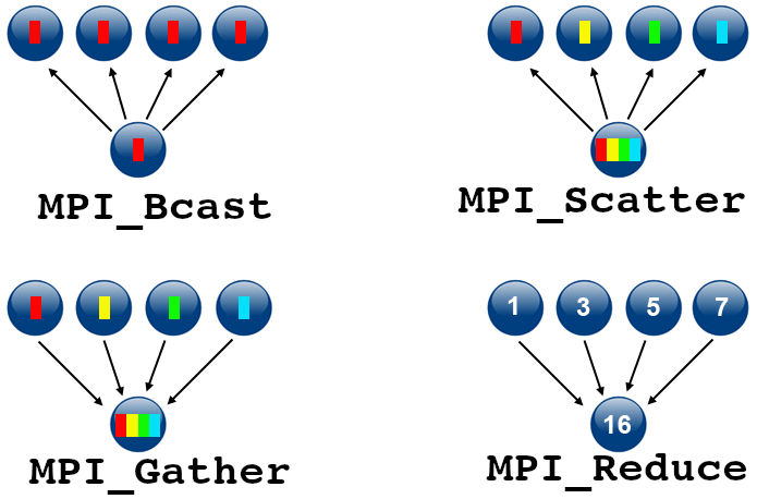 Collective Communications
The MPI_Bcast and MPI_Reduce operations have more complex analogs that are very useful in a variety of algorithms.
Just like MPI_Bcast and MPI_Reduce, the benefit of using these routines, instead of point-to-point messages, is not only syntactical convenience but also much better efficiency.
They allow for swaths of data to be distributed from a root process to all other available processes, or data from all processes can be collected at one process.
These operators can eliminate the need for a surprising amount of boilerplate code via two functions:
Keep in mind that these are called “collective” because every PE in the communicator must call these routines at the same time.
Let’s take a look at the basic idea, and then we’ll see the wide variety of related routines.
USE mpi_f08
MPI_Scatter(sendbuf, sendcount, sendtype, recvbuf, recvcount, recvtype,
        root, comm, ierror)
    TYPE(*), DIMENSION(..), INTENT(IN) :: sendbuf
    TYPE(*), DIMENSION(..) :: recvbuf
    INTEGER, INTENT(IN) :: sendcount, recvcount, root
    TYPE(MPI_Datatype), INTENT(IN) :: sendtype, recvtype
    TYPE(MPI_Comm), INTENT(IN) :: comm
    INTEGER, OPTIONAL, INTENT(OUT) :: ierror

MPI_Gather(sendbuf, sendcount, sendtype, recvbuf, recvcount, recvtype,
        root, comm, ierror)
    TYPE(*), DIMENSION(..), INTENT(IN) :: sendbuf
    TYPE(*), DIMENSION(..) :: recvbuf
    INTEGER, INTENT(IN) :: sendcount, recvcount, root
    TYPE(MPI_Datatype), INTENT(IN) :: sendtype, recvtype
    TYPE(MPI_Comm), INTENT(IN) :: comm
    INTEGER, OPTIONAL, INTENT(OUT) :: ierror
In order to get a better grasp on these functions, let’s go ahead and create a program that will utilize the scatter function. Note that the gather function (not shown in the example) works similarly, and is essentially the converse of the scatter function. Further examples which utilize the gather function can be found in the MPI tutorials listed as resources at the beginning of this document.
Example of Scatter
This example shows how to spread the values of a 2 dimensional array across multiple processes
program scatter
   use mpi_f08

   integer, parameter :: nsize = 8
   integer :: numtasks, rank, sendcount, recvcount, source, ierr
   real, allocatable ::  sendbuf(:, :), recvbuf(:)

   call MPI_INIT(ierr)
   call MPI_COMM_RANK(MPI_COMM_WORLD, rank, ierr)
   call MPI_COMM_size(MPI_COMM_WORLD, numtasks, ierr)

   allocate (sendbuf(nsize, numtasks))
   allocate (recvbuf(nsize))
   sendbuf = reshape([(i, i=1, nsize*numtasks)], [nsize, numtasks])

   if (rank == 0) then
      print *, ''
      print *, 'Original array to be distributed:'
      do i = 1, numtasks
         print *, sendbuf(:, i)
      end do
      print *, ''
   end if

   call MPI_BARRIER(MPI_COMM_WORLD)

   source = 1
   sendcount = nsize
   recvcount = nsize
   call MPI_SCATTER(sendbuf, sendcount, MPI_REAL, recvbuf, recvcount, MPI_REAL, &
                    source, MPI_COMM_WORLD, ierr)

   print *, 'rank= ', rank, ' recvbuf: ', recvbuf

   call MPI_FINALIZE(ierr)

   deallocate (sendbuf, recvbuf)

end program
Group and Communicator Management Routines
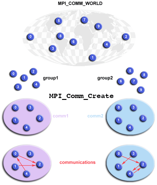 Groups and Communications
Groups and Communicators
A group is an ordered set of processes. Each process in a group is associated with a unique integer rank. Rank values start at zero and go to N-1, where N is the number of processes in the group. In MPI, a group is represented within system memory as an object. It is accessible to the programmer only by a “handle”. A group is always associated with a communicator object.
A communicator encompasses a group of processes that may communicate with each other. All MPI messages must specify a communicator. In the simplest sense, the communicator is an extra “tag” that must be included with MPI calls. Like groups, communicators are represented within system memory as objects and are accessible to the programmer only by “handles”. For example, the handle for the communicator that comprises all tasks is MPI_COMM_WORLD.
From the programmer’s perspective, a group and a communicator are one. The group routines are primarily used to specify which processes should be used to construct a communicator.
Primary Purposes of Group and Communicator Objects:
- Allow you to organize tasks, based upon function, into task groups.
- Enable Collective Communications operations across a subset of related tasks.
- Provide basis for implementing user defined virtual topologies.
- Provide for safe communications.
Programming Considerations and Restrictions:
Groups/communicators are dynamic - they can be created and destroyed during program execution.
Processes may be in more than one group/communicator. They will have a unique rank within each group/communicator.
MPI provides over 40 routines related to groups, communicators, and virtual topologies.
Typical usage:
- Extract handle of global group from MPI_COMM_WORLD using MPI_Comm_group
- Form new group as a subset of global group using MPI_Group_incl
- Create new communicator for new group using MPI_Comm_create
- Determine new rank in new communicator using MPI_Comm_rank
- Conduct communications using any MPI message passing routine
- When finished, free up new communicator and group (optional) using MPI_Comm_free and MPI_Group_free
Example of a use of Groups
program group
   use mpi_f08

   implicit none

   integer :: nsize, i
   integer :: rank, new_rank, sendbuf, recvbuf, numtasks, ierr
   integer, dimension(:), allocatable :: ranks1(:), ranks2(:)
   type(MPI_Group) :: orig_group, new_group  ! MPI 3.0
   type(MPI_Comm) :: new_comm

   call MPI_INIT(ierr)
   call MPI_COMM_RANK(MPI_COMM_WORLD, rank, ierr)
   call MPI_COMM_SIZE(MPI_COMM_WORLD, numtasks, ierr)

   if (mod(numtasks, 2) /= 0) then
      print *, 'Enter a even number of processes '
      call MPI_FINALIZE(ierr)
      stop
   end if

   allocate (ranks1(numtasks/2))
   allocate (ranks2(numtasks/2))

   ranks1 = [(i, i=0, size(ranks1) - 1)]
   ranks2 = [(size(ranks1) + i, i=0, size(ranks2) - 1)]

   sendbuf = rank

   ! extract the original group handle
   call MPI_COMM_GROUP(MPI_COMM_WORLD, orig_group, ierr)

   ! divide tasks into two distinct groups based upon rank
   if (rank < numtasks/2) then
       call MPI_GROUP_INCL(orig_group, numtasks/2, ranks1, new_group, ierr)
   else
       call MPI_GROUP_INCL(orig_group, numtasks/2, ranks2, new_group, ierr)
   end if

   ! create new new communicator and then perform collective communications
   call MPI_COMM_CREATE(MPI_COMM_WORLD, new_group, new_comm, ierr)
   call MPI_ALLREDUCE(sendbuf, recvbuf, 1, MPI_INTEGER, MPI_SUM, new_comm, ierr)

   ! get rank in new group
   call MPI_GROUP_RANK(new_group, new_rank, ierr)
   print *, 'rank= ', rank, ' newrank= ', new_rank, ' recvbuf= ', recvbuf

   call MPI_FINALIZE(ierr)
end program
Key Points
Collective operations are usually more efficient than point-to-point messages
Exercises
Overview
Teaching: 0 min
Exercises: 60 minQuestions
Objectives
Exercise 1
Write a Fortran code that print its rank and total number of processes in the communicator.
Exercise 2:
Write a Fortran code that computes the integral of function
f(x)=log(pix)sin(pi*x)**2 + x in the range [1,10]
distributing the rectangles across multiple processes using MPI
Exercise 3:
Write a Fortran code that distributes a long array of random numbers and use each process will compute the average value of the section of the array allocated.
Use collective operations to return the maximum and minimum of those averages.
Key Points
Final
Overview
Teaching: min
Exercises: minQuestions
Objectives
Use the break layout for placeholder episodes representing coffee breaks and lunches.
These episodes do not have exercises, questions, objectives, or keypoints in their metadata,
but must have a “break” field to show how long the break is (in minutes).
Key Points