Overview

Teaching: 60 min
Exercises: 0 min

Questions

• How to get faster executions using more cores, GPUs or machines.

Objectives

• Learn the most commonly used parallel programming paradigms

Why Parallel Computing?

Since around the 90s, Fortran designers understood that the era of programming for a single CPU will be abandoned very soon. At that time, vector machines exist but they were in use for very specialized calculations. It was around 2004 that the consumer market start moving out of having a single fast CPU with a single processing unit into a CPU with multiple processing units or cores. Many codes are intrinsically serial and adding more cores did not bring more performance out of those codes. The figure below shows how a serial code today runs 12 times slower than it could if the increase in performance could have continued as it were before 2004. That is the same as saying that the code today runs at a speed that could have been present 8 to 10 years ago with if the trend could have been sustained up to now.

The reason for this lack is not a failure in Moore’s law when measured in the number of transistors on CPUs.

The fact is that instead of faster CPUs computers today have more cores on each CPU, machines on HPC clusters have 2 or more CPU sockets on a single mainboard and we have Accelerators, machines with massive amounts of simple cores that are able to perform certain calculations more efficiently than contemporary CPU.

It should be clear that computers today are not getting faster and faster over the years as was the case during the 80s and 90s. Computers today are just getting marginally faster if you look at one individual core, but today we have more cores on a machine and basically, every computer, tablet, and phone around us is a multiprocessor.

It could be desirable that parallelism could be something that a computer deals with automatically. The reality is that today, writing parallel code or converting serial code, ie codes that are supposed to run on a single core is not a trivial task.

Parallel Programming in Fortran

After the release of Fortran 90 parallelization at the level of the language was considered. High-Performance Fortran (HPF) was created as an extension of Fortran 90 with constructs that support parallel computing, Some HPF capabilities and constructs were incorporated in Fortran 95. The implementation of HPF features was uneven across vendors and OpenMP attracts vendors to better support OpenMP over HPF features. In the next sections, we will consider a few important technologies that bring parallel computing to the Fortran Language. Some like coarrays are part of the language itself, like OpenMP, and OpenACC, are directives added as comments to the sources and compliant compilers can use those directives to provide parallelism. CUDA Fortran is a superset of the Fortran language and MPI a library for distributed parallel computing. In the following sections a brief description of them.

Fortran coarrays

One of the original features that survived was coarrays. Coarray Fortran (CAF), started as an extension of Fortran 95/2003 but it reach a more mature standard in Fortran 2008 with some modifications in 2018.

The following example is our simple code for computing pi written using coarrays. (example_01.f90)

program pi_coarray

   use iso_fortran_env
   implicit none

   integer, parameter :: r15 = selected_real_kind(15)
   integer, parameter :: n = huge(1)
   real(kind=r15), parameter :: pi_ref = 3.1415926535897932384626433_real64

   integer :: i
   integer :: n_per_image[*]
   real(kind=r15) :: real_n[*]
   real(kind=r15) :: pi[*] = 0.0
   real(kind=r15) :: t[*]

   if (this_image() .eq. num_images()) then
      n_per_image = n/num_images()
      real_n = real(n_per_image*num_images(), r15)

      print *, 'Number of terms requested : ', n
      print *, 'Real number of terms      : ', real_n
      print *, 'Terms to compute per image: ', n_per_image
      print *, 'Number of images          : ', num_images()
      do i = 1, num_images() - 1
         n_per_image[i] = n_per_image
         real_n[i] = real(n_per_image*num_images(), r15)
      end do

   end if

   sync all

   ! Computed on each image
   do i = (this_image() - 1)*n_per_image, this_image()*n_per_image - 1
      t = (real(i) + 0.05)/real_n
      pi = pi + 4.0/(1.0 + t*t)
   end do

   sync all

   if (this_image() .eq. num_images()) then

      do i = 1, num_images() - 1
         !print *, pi[i]/real_n
         pi = pi + pi[i]
      end do

      print *, "Computed value", pi/real_n
      print *, "abs difference with reference", abs(pi_ref - pi/n)
   end if

end program pi_coarray

You can compile this code using the Intel Fortran compiler which offers integrated support for Fortran coarrays in shared memory. If you are using environment modules be sure of loading modules for the compiler and the MPI implementation. Intel MPI is needed as the intel implementation of coarrays is build on top of MPI.

$> module load compiler mpi

$> $ ifort -coarray example_01.f90

$> time ./a.out 
 Number of terms requested :   2147483647
 Real number of terms      :    2147483616.00000     
 Terms to compute per image:     44739242
 Number of images          :           48
 Computed value   3.14159265405511     
 abs difference with reference  4.488514004918898E-008

real    0m2.044s
user    0m40.302s
sys     0m16.386s

Another alternative is using gfortran using the OpenCoarrays implementation. For a cluster using modules, you need to load the GCC compiler, a MPI implementation and the module for opencoarrays.

$> module load lang/gcc/11.2.0 parallel/openmpi/3.1.6_gcc112 libs/coarrays/2.10.1_gcc112_ompi316 

There are two ways of compile and run the code. OpenCoarrays has its own wrapper for the compiler and executor.

$> caf example_01.f90

To execute the resulting binary use the cafrun command.

$> time cafrun -np 24 ./a.out
 Number of terms requested :   2147483647
 Real number of terms      :    2147483640.0000000     
 Terms to compute per image:     89478485
 Number of images          :           24
 Computed value   3.1415926540550383     
 abs difference with reference   9.7751811090063256E-009

real    1m32.622s
user    36m29.776s
sys     0m9.890s

Another alternative is to explicitly compile and run

$> $ gfortran -fcoarray=lib example_01.f90 -lcaf_mpi

And execute using mpirun command:

$ time mpirun -np 24 ./a.out 
 Number of terms requested :   2147483647
 Real number of terms      :    2147483640.0000000     
 Terms to compute per image:     89478485
 Number of images          :           24
 Computed value   3.1415926540550383     
 abs difference with reference   9.7751811090063256E-009

real    1m33.857s
user    36m26.924s
sys     0m11.614s

When the code runs, multiple processes are created, each of them is called an image. They execute the same executable and the processing could diverge by using a unique number that can be inquired with the intrinsic function this_image(). In the example above, we distribute the terms in the loop across all the images. Each image computes different terms of the series and store the partial sum in the variable pi. The variable pi is defined as a coarray with using the [*] notation. That means that each individual has its own variable pi but still can transparently access the value from other images.

At the end of the calculation, the last image is collecting the partial sum from all other images and returns the value obtained from that process.

OpenMP

OpenMP was conceived originally as an effort to create a standard for shared-memory multiprocessing (SMP). Today, that have changed to start supporting accelerators but the first versions were concerned only with introducing parallel programming directives for multicore processors.

With OpenMP, you can go beyond the directives and use an API, using methods and routines that explicitly demand the compiler to be compliant with those parallel paradigms.

One of the areas where OpenMP is easy to use is parallelizing loops, same as we did use coarrays and as we will be doing as example for the other paradigms of parallelism.

As an example, lets consider the same program used to introduce Fortran. The algorithm computes pi using a quadrature. (example_02.f90)

program converge_pi

   use iso_fortran_env

   implicit none

   integer, parameter :: knd = max(selected_real_kind(15), selected_real_kind(33))
   integer, parameter :: n = huge(1)/1000
   real(kind=knd), parameter :: pi_ref = 3.1415926535897932384626433832795028841971_knd

   integer :: i
   real(kind=knd) :: pi = 0.0, t

   print *, 'KIND      : ', knd
   print *, 'PRECISION : ', precision(pi)
   print *, 'RANGE     : ', range(pi)

   !$OMP PARALLEL DO PRIVATE(t) REDUCTION(+:pi)
   do i = 0, n - 1
      t = real(i + 0.5, kind=knd)/n
      pi = pi + 4.0*(1.0/(1.0 + t*t))
   end do
   !$OMP END PARALLEL DO

   print *, ""
   print *, "Number of terms in the series : ", n
   print *, "Computed value : ", pi/n
   print *, "Reference vaue : ", pi_ref
   print *, "ABS difference with reference : ", abs(pi_ref - pi/n)

end program converge_pi

This code is almost identical to the original code the only difference resides on a couple of comments before and after the loop:

!$OMP PARALLEL DO PRIVATE(t) REDUCTION(+:pi)
do i = 0, n - 1
   t = real(i + 0.5, kind=knd)/n
   pi = pi + 4.0*(1.0/(1.0 + t*t))
end do
!$OMP END PARALLEL DO

These comments are safely ignored by a compiler that does not support OpenMP. A compiler supporting OpenMP will use those instructions to create an executable that will span a number of threads. Each thread could potentially run on independent cores resulting on the parallelization of the loop. OpenMP also includes features to collect the partial sums of pi.

To compile this code each compiler provides arguments that enable the support for it. In the case of GCC the compilation is:

$> gfortran -fopenmp example_02.f90

For the Intel compilers the argument is -qopenmp

$> ifort -qopenmp example_02.f90

On the NVIDIA Fortran compiler the argument is -mp. The extra argument -Minfo=all is very useful to receive feedback from the compiler about sections of the code that will be parallelized.

$> nvfortran -mp -Minfo=all example_02.f90

OpenACC

OpenACC is another directive-based standard for parallel programming. OpenACC was created with to facilitate parallelism not only for multiprocessors but also for external accelerators such as GPUs.

Same as OpenMP, in OpenACC the programming is carried out by adding some extra lines to the serial code that are comments from the point of view of the language but are interpreted by a compliant language that is capable of interpreting those lines and parallelizing the code according to them. The lines of code added to the original sources are called directives. An ignorant compiler will just ignore those lines and the code will execute as before the introduction of the directives.

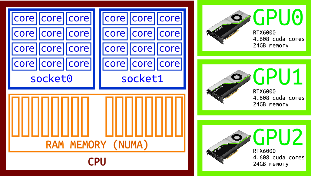
An accelerator is a device specialized on certain numerical operations. It usually includes an independent memory device and data needs to be transferred to the device’s memory before the accelerator can process the data. The figure below show a schematic of one multicore machine with 3 GPUs attached to it.

As we did for OpenMP, the same code can be made parallel by adding a few directives. (example_03.f90)

program converge_pi

   use iso_fortran_env

   implicit none

   integer, parameter :: knd = max(selected_real_kind(15), selected_real_kind(33))
   integer, parameter :: n = huge(1)/1000
   real(kind=knd), parameter :: pi_ref = 3.1415926535897932384626433832795028841971_knd

   integer :: i
   real(kind=knd) :: pi = 0.0, t

   print *, 'KIND      : ', knd
   print *, 'PRECISION : ', precision(pi)
   print *, 'RANGE     : ', range(pi)

   !$ACC PARALLEL LOOP PRIVATE(t) REDUCTION(+:pi)
   do i = 0, n - 1
      t = real(i + 0.5, kind=knd)/n
      pi = pi + 4.0*(1.0/(1.0 + t*t))
   end do
   !$ACC END PARALLEL LOOP

   print *, ""
   print *, "Number of terms in the series : ", n
   print *, "Computed value : ", pi/n
   print *, "Reference vaue : ", pi_ref
   print *, "ABS difference with reference : ", abs(pi_ref - pi/n)

end program converge_pi

The loop is once more surrounded by directives that for this particular case looks very similar to the OpenMP directives presented before.

!$ACC PARALLEL LOOP PRIVATE(t) REDUCTION(+:pi)
do i = 0, n - 1
   t = real(i + 0.5, kind=knd)/n
   pi = pi + 4.0*(1.0/(1.0 + t*t))
end do
!$ACC END PARALLEL LOOP

For the OpenACC version of the code the compilation line is:

$> gfortran -fopenacc example_03.f90

Intel compilers do not support OpenACC The best support comes from NVIDIA compilers

$> nvfortran -acc -Minfo=all example_03.f90

Using directives instead of extending the language offers several advantages:

• The original source code continues to be valid for those compilers that do know about OpenMP or OpenACC, there is no need to fork the code. If you stay at the level of directives, the code will continue to work without parallelization.

• The directives provide a very high-level abstraction for parallelism. Other solutions involve deep knowledge about the architecture where the code will run reducing the portability to other systems. Architectures evolve over time and hardware specifics will become a burden for maintainers of the code when it needs to be adapted to newer technologies.

• The parallelization effort can be done step by step. There is no need to start from scratch planning important rewrites of large portions of the code with will come with more bugs and development costs.

An alternative to OpenMP could be pthreads, and an alternative to OpenACC could be CUDA. Both alternatives suffer from the items mentioned above.

Despite of the similarities at this point, OpenMP and OpenACC were created targeting very different architectures. The idea is that eventually, both will converge into a more general solution. We will now discuss each approach separately, at the end of this discussion we will talk about the efforts to converge both approaches.

Key Points

• Use OpenMP for multiple cores, OpenACC and CUDA Fortran for GPUs and MPI for distributed computing.