Introduction
Overview
Teaching: 30 min
Exercises: 30 minQuestions
What is High-Performance Computing?
What is a HPC cluster or Supercomputer?
How my computer compares with a HPC cluster?
Learn the components of the HPC
Learn the basic terminology in HPC
High Performance Computing
High-Performance Computing is about size and speed. A HPC cluster is made of tens, hundreds or even thousands of relatively normal computers specially connected to perform intensive computational operations. In most cases those operations involve large numerical calculations that take too much time to complete and therefore are simply unfeasible to perform on a normal machine.
This is a very pragmatic tutorial: more time on examples and exercises, less time on theoretical stuff. The idea is that after these lessons, you will have learned how to enter into the cluster, compile code, execute using the queue system and transfer data in an out the cluster.
What are the specifications of my own computer?
Check your computer, gather information about the CPU, number of Cores, Total RAM memory and Hard Drive.
The purpose of this exercise is to compare your machine with our clusters
You can see specs for our clusters Spruce Knob and Thorny Flat
Try to gather an idea on the Hardware present on your machine and see the hardware we have on Spruce Knob or Thorny Flat
Here are some tricks to get that data from several Operating Systems
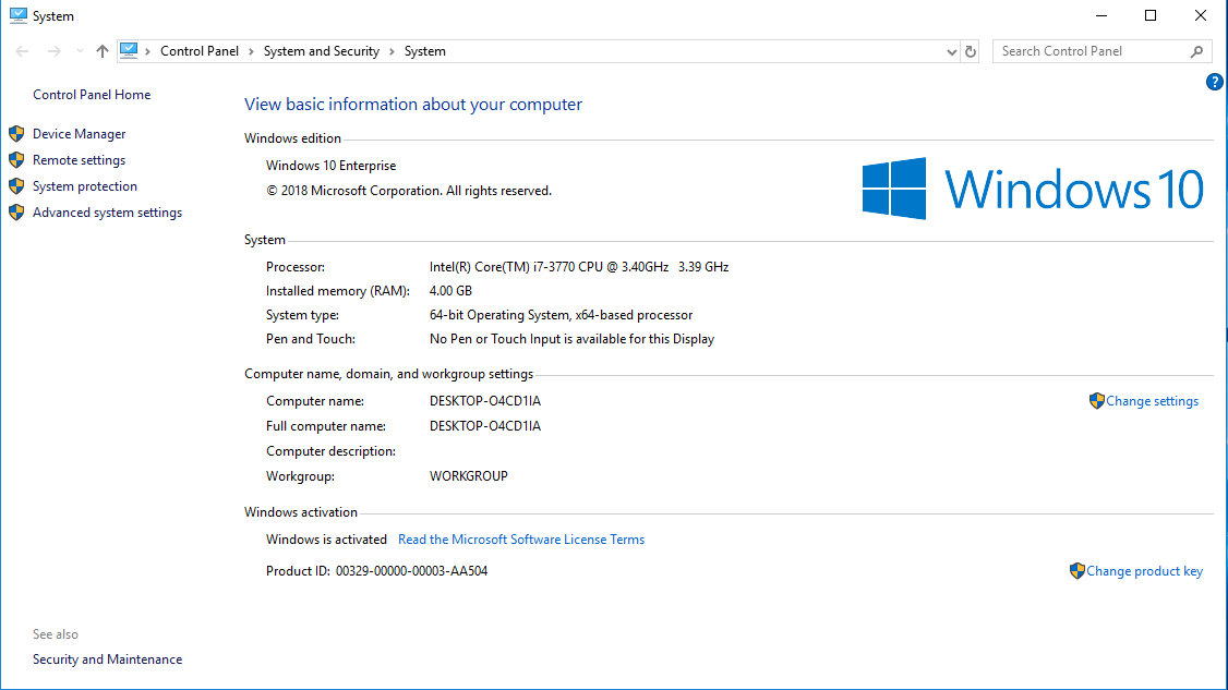
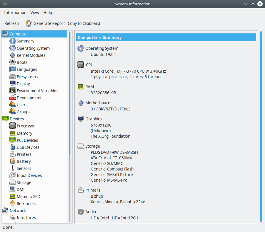
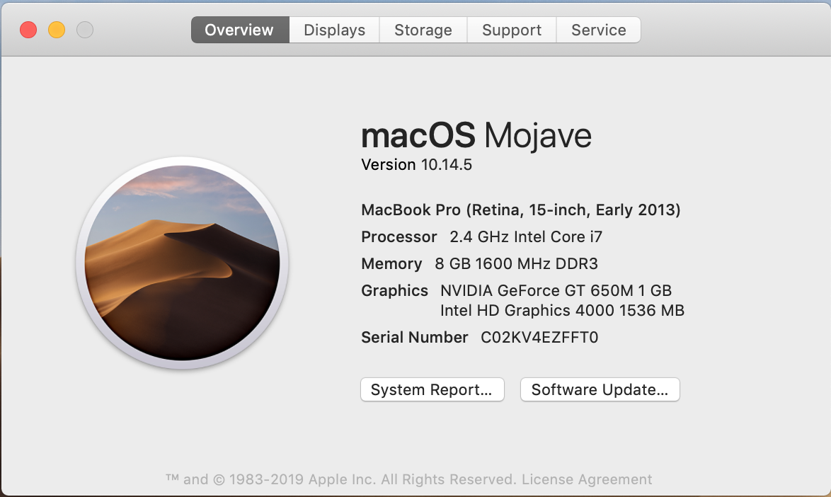 If you want more data click on "System Report..." and you will get:
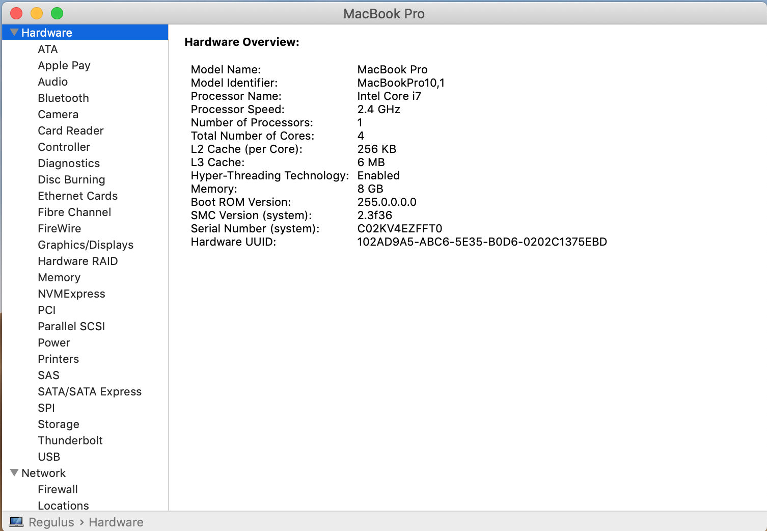
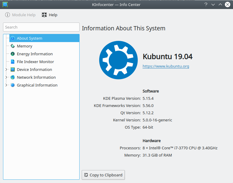
In Linux gathering the data from a GUI depends a lot from more from the exact distribution you are using here some tools that you can try
KDE Info Center
Linux Mint Cinnamon System Info
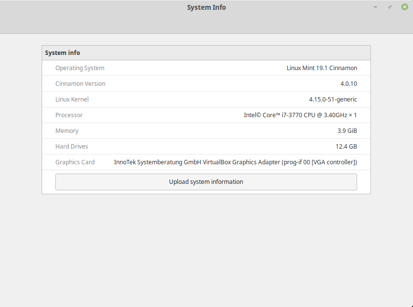
Linux Mint Cinnamon System Info
Central Processing Units
CPU Brands and Product lines
There are only two manufacturers that hold most of the market for PC consumer computing: Intel and AMD. There are several others manufacturers of CPUs but those are mostly for Smart Phones, Photo Cameras, Musical Instruments, or very specialized HPC clusters and equipment.
More than a decade ago, the main feature used for marketing purposes on a CPU was the speed. That has changed now as CPUs are not getting much faster due to faster clock speed. It is hard to market the performance of a new processor with a single number. That is why CPUs are now marketed with “Product Lines” and the “Model numbers” those number bear no direct relation with the actual characteristics of a given processor.
For example, Intel Core i3 processors are marketed for entry level machines more tailored to basic computing tasks like word processing and web browsing. On the other hand, Intel’s Core i7 and i9 processors are for high-end products aimed at the top of the line gaming machines able to run the most recent titles at high FPS and resolutions. Machines for enterprise usage are usually under the Xeon Line.
On AMD’s side, you have the Athlon line aimed at entry-level users, From Ryzen(TM) 3 for basic applications, all the way to the Ryzen(TM) 9 designed mostly for enthusiasts and gamers. AMD also has product lines for enterprises like EPYC Server Processors.
Cores
Consumer level CPUs up to 2000s only had one core, but Intel and AMD both hit a brick wall with incremental clock speeds improvements. The heat and power consumption scales non-linearly with the CPU speed. That brings us to the current trend and instead of a single core, CPUs now have two, three, four, eight or sixteen cores on a single CPU. That means that each CPU (in marketing terms) is actually several CPUs (in actual component terms).
Hyperthreading
Hyperthreading is intrinsically linked to cores and is best understood as a proprietary technology that allows the operating system, to recognize the CPU as having double the amount of cores.
In practical terms, a CPU with four physical cores would be recognized by the operating system as having eight virtual cores, or capable of dealing with eight threads of execution. The idea is that by doing that it is expected that the CPU is able to better manage the extra load, by reordering execution and pipelining the workflow to the actual number of physical cores.
In the context of HPC there is still debate if activating Hyperthreading is beneficial for intensive numerical operations and the answer is very dependent on the code. In our clusters Hyperthreading is disabled on all compute nodes and enabled on service nodes.
CPU Frequency
Back in the 80s and 90s CPU frequency was the most important feature of a CPU or at least that was the way it was marketed.
Other names for CPU frequency are “clock rate”, or “clock speed”. CPUs work by steps instead of continuous flow of information. The speed of the CPU is today measured in GHz, or how quickly the processor can process instructions in any given second (clock cycles per second). 1 Hz equals one cycle per second, so a 2 GHz frequency can handle 2 billion instructions for every second.
The higher the frequency the more operations can be done. However, today that is not the whole story. Modern CPUs have complex CPU extensions (SSE, AVX, AVX2 and AVX512) that allow the CPU to execute several numerical operations on a single clock step.
From another side, CPUs are now able to change the speed up to certain limits, raising and lowering the value if needed. Sometimes raising the CPU frequency of a multicore CPU means that some cores are disabled as result.
Another technique used often by gamers is overclocking. Overclocking, is when the frequency is altered beyond the manufacturer’s official clock rate by user-generated means. In HPC this is often not applied as overclocking increases the chances of instability of the system.
Cache
Cache is a high-speed momentary memory format assigned to the CPU to facilitate future retrieval of data and instructions before processing. It’s very similar to RAM in the sense that it acts as a temporary holding pen for data. However CPU’s access this memory in chunks and the mapping to RAM is different.
Contrary to RAM that are independent pieces of hardware, cache sits on the CPU itself, so the access times are significantly faster. The cache is an important portion of the production cost of a CPU, to the point where one of the differences between i3s, i5s, and i7s is basically the size of the cache memory.
There are actually several cache memories inside a CPU. They are called cache levels, or hierarchies, a bit like a pyramid: L1, L2, and L3. The lower the level the closer to the core.
From the HPC perspective for intensive numerical operations, the cache size is an important feature. Many CPU cycles are lost if you need to bring data all the time from the RAM or even worst from the Hard Drive. So having large amounts of cache improves the efficiency of HPC codes.
Learn to read computer specifications
One of the central differences between one computer and another are the CPU, the chip or set of chips that control most of the numerical operations. When reading the specifications of a computer you need to pay attention to the amount of memory, if the drive is SSD or not, the presence of a dedicated GPU card and a number of factors that could or could not be relevant for the purpose of your computer. Have a look at the specifications of the CPU on your machine.
Intel
If your machine uses Intel Processors, go to https://ark.intel.com and enter the model of CPU you have, Intel models are for example: “E5-2680 v3”, “E5-2680 v3”
AMD
If your machine uses AMD processors, go to https://www.amd.com/en/products/specifications/processors and check the details for your machine.
Key Points
Learn about CPUs, cores, and cache, and comparing your own machine with an HPC cluster
The Command Line Interface
Overview
Teaching: 60 min
Exercises: 30 minQuestions
How to use the Linux terminal
Objectives
Learn the basic commands
Command Line Interface
At a high level, a HPC cluster is a big computer to be used by several users at the same time. The users expect to run a variety of scientific codes, store the data needed as input or generated as output. In HPC, computers usually communicate with each other for tasks that are too big for a single computer to deal and interact with us allowing us to make decisions and see errors.
Our interaction with computers happens in many different ways, including through a keyboard and mouse, touch screen interfaces, or using speech recognition systems. However in HPC we need an efficient and still very light way of communicating with the head node. The front end machine in a HPC cluster. In contrast Desktop computers uses a Graphical User Interface.
The graphical user interface (GUI) is the most widely used way to interact with personal computers. We give instructions (to run a program, to copy a file, to create a new folder/directory) with the convenience of a few mouse clicks. This way of interacting with a computer is intuitive and very easy to learn. But this way of giving instructions to a computer scales very poorly if we are to give a large stream of instructions even if they are similar or identical. For example if we have to copy the third line of each of a thousand text files stored in thousand different directories and paste it into a single file line by line. Using the traditional GUI approach of clicks will take several hours to do this.
This is where we take advantage of the shell - a command-line interface to make such repetitive tasks automatic and fast. It can take a single instruction and repeat it as is or with some modification as many times as we want. The task in the example above can be accomplished in a few minutes at most.
The heart of a command-line interface is a read-evaluate-print loop (REPL). It is called so because when you type a command and press Return (also known as Enter) the shell reads your command, evaluates (or “executes”) it, prints the output of your command, loops back and waits for you to enter another command.
The Shell
The Shell is a program which runs other programs rather than doing calculations itself. Those programs can be as complicated as climate modeling software and as simple as a program that creates a new directory. The simple programs which are used to perform stand alone tasks are usually refered to as commands. The most popular Unix shell is Bash, (the Bourne Again SHell — so-called because it’s derived from a shell written by Stephen Bourne). Bash is the default shell on most modern implementations of Unix and in most packages that provide Unix-like tools for Windows.
When the shell is first opened, you are presented with a prompt, indicating that the shell is waiting for input.
$
The shell typically uses $ as the prompt, but may use a different symbol.
We’ll show the prompt in several ways, mostly as $ but you can see other versions like $> or [training001@srih0001 ~]$ . The last one is the default prompt for the user training001 at the Spruce head node.
Most importantly: when typing commands, either from these lessons or from other sources, do not type the prompt, only the commands that follow it.
So let’s try our first command, which will list the contents of the current directory:
[training001@srih0001 ~]$ ls -al
total 64
drwx------   4 training001 training   512 Jun 27 13:24 .
drwxr-xr-x 151 root        root     32768 Jun 27 13:18 ..
-rw-r--r--   1 training001 training    18 Feb 15  2017 .bash_logout
-rw-r--r--   1 training001 training   176 Feb 15  2017 .bash_profile
-rw-r--r--   1 training001 training   124 Feb 15  2017 .bashrc
-rw-r--r--   1 training001 training   171 Jan 22  2018 .kshrc
drwxr-xr-x   4 training001 training   512 Apr 15  2014 .mozilla
drwx------   2 training001 training   512 Jun 27 13:24 .ssh
Command not found
If the shell can’t find a program whose name is the command you typed, it will print an error message such as:
$ ksks: command not foundUsually this means that you have mis-typed the command.
Why use the CLI?
The Command Line Interface was one of the first ways of interacting with computers. Previously the interaction happened with perforated cards or even switching cables on a big console. Still the CLI is a powerful way of talking with computers.
It is a different model of interacting than a GUI, and that will take some effort - and some time - to learn. A GUI presents you with choices and you select one. With a command line interface (CLI) the choices are combinations of commands and parameters, more like words in a language than buttons on a screen. They are not presented to you so you must learn a few, like learning some vocabulary in a new language. But a small number of commands gets you a long way, and we’ll cover those essential few today.
Flexibility and automation
The grammar of a shell allows you to combine existing tools into powerful pipelines and handle large volumes of data automatically. Sequences of commands can be written into a script, improving the reproducibility of workflows and allowing you to repeat them easily.
In addition, the command line is often the easiest way to interact with remote machines and supercomputers. Familiarity with the shell is near essential to run a variety of specialized tools and resources including high-performance computing systems. As clusters and cloud computing systems become more popular for scientific data crunching, being able to interact with the shell is becoming a necessary skill. We can build on the command-line skills covered here to tackle a wide range of scientific questions and computational challenges.
Exercise 1
Commands in Unix/Linux are very stable with some commands being around for decades now. So what your learn will be of good use in the future. This exercises pretend to give you a feeling of the different parts of a command.
Execute the command cal, we executed that in our previous episode. Execute it again like this cal -y. You should get an output like this:
[training001@srih0001 ~]$ cal -y
                               2019

       January               February                 March
Su Mo Tu We Th Fr Sa   Su Mo Tu We Th Fr Sa   Su Mo Tu We Th Fr Sa
       1  2  3  4  5                   1  2                   1  2
 6  7  8  9 10 11 12    3  4  5  6  7  8  9    3  4  5  6  7  8  9
13 14 15 16 17 18 19   10 11 12 13 14 15 16   10 11 12 13 14 15 16
20 21 22 23 24 25 26   17 18 19 20 21 22 23   17 18 19 20 21 22 23
27 28 29 30 31         24 25 26 27 28         24 25 26 27 28 29 30
                                              31
        April                   May                   June
Su Mo Tu We Th Fr Sa   Su Mo Tu We Th Fr Sa   Su Mo Tu We Th Fr Sa
    1  2  3  4  5  6             1  2  3  4                      1
 7  8  9 10 11 12 13    5  6  7  8  9 10 11    2  3  4  5  6  7  8
14 15 16 17 18 19 20   12 13 14 15 16 17 18    9 10 11 12 13 14 15
21 22 23 24 25 26 27   19 20 21 22 23 24 25   16 17 18 19 20 21 22
28 29 30               26 27 28 29 30 31      23 24 25 26 27 28 29
                                              30
        July                  August                September
Su Mo Tu We Th Fr Sa   Su Mo Tu We Th Fr Sa   Su Mo Tu We Th Fr Sa
    1  2  3  4  5  6                1  2  3    1  2  3  4  5  6  7
 7  8  9 10 11 12 13    4  5  6  7  8  9 10    8  9 10 11 12 13 14
14 15 16 17 18 19 20   11 12 13 14 15 16 17   15 16 17 18 19 20 21
21 22 23 24 25 26 27   18 19 20 21 22 23 24   22 23 24 25 26 27 28
28 29 30 31            25 26 27 28 29 30 31   29 30

       October               November               December
Su Mo Tu We Th Fr Sa   Su Mo Tu We Th Fr Sa   Su Mo Tu We Th Fr Sa
       1  2  3  4  5                   1  2    1  2  3  4  5  6  7
 6  7  8  9 10 11 12    3  4  5  6  7  8  9    8  9 10 11 12 13 14
13 14 15 16 17 18 19   10 11 12 13 14 15 16   15 16 17 18 19 20 21
20 21 22 23 24 25 26   17 18 19 20 21 22 23   22 23 24 25 26 27 28
27 28 29 30 31         24 25 26 27 28 29 30   29 30 31
The command line is powerful enough to allow you to even do programming. Execute this command and see the answer
[training001@srih0001 ~]$ n=1; while test $n -lt 10000; do echo $n; n=`expr 2 \* $n`; done
1
2
4
8
16
32
64
128
256
512
1024
2048
4096
8192
If you are not getting this output check the command line very carefully. Even small changes could be interpreted by the shell as entirely different commands so you need to be extra careful and gather insight when commands are not doing what you want.
The echo and cat commands
Your fist command will show you what those locations are. Execute:
$> echo $HOME
/users/<username>
$> echo $SCRATCH
/scratch/<username>
The first command to learn is echo. The command above uses echo to
show the contents of two shell variables $HOME and $SCRATCH. Shell
variables are ways to store information in such a way that the shell can
use it when needed. Each user on the cluster receives appropriated
values for those variables.
Let us explore a bit more the usage of echo. Enter this command line
and execute ENTER:
$> echo "I am learning UNIX Commands"
I am learning UNIX Commands
The shell is actually able to do basic arithmetical operations, execute this command:
$> echo $((23+45*2))
113
Notice that as customary in mathematics products take precedence over addition. That is called the PEMDAS order of operations, ie "Parentheses, Exponents, Multiplication and Division, and Addition and Subtraction". Check your understanding of the PEMDAS rule with this command:
$> echo $(((1+2**3*(4+5)-7)/2+9))
42
Notice that the exponential operation is expressed with the **
operator. The usage of echo is important, otherwise, if you execute
the command without echo the shell will do the operation and will try
to execute a command called 42 that does not exist on the system. Try
by yourself:
$> $ $(((1+2**3*(4+5)-7)/2+9))
-bash: 42: command not found
As you have seen before, when you execute a command on the terminal in most cases you see the output printed on the screen. The next thing to learn is how to redirect the output of a command into a file. This will be very important later to submit jobs and control where and how the output is produced. Execute the following command:
$> echo "I am learning UNIX Commands" > report.log
With the character > redirects the output from echo into a file
called report.log. No output is printed on the screen. If the file
does not exist it will be created. If the file exists previously, the
file is erased and only the new contents are stored.
To check that the file actually contains the line produced by echo, execute:
$> cat report.log
I am learning UNIX Commands
The cat (concatenate) command displays the contents of one or several files. In the case of multiple files the files are printed in the order they are described in the command line, concatenating the output so the name of the command.
You can even use a nice trick to write a small text on a file. Execute
the following command, followed by the text that you want to write, at
the end execute Ctrl-D (^D), the Control Key followed by the D
key. I am annotating below the location where ^D should be executed:
$> cat > report.log
I am learning UNIX Commands^D
$> cat report.log
I am learning UNIX Commands
In fact, there are hundreds of commands, most of them with a variety of options that change the behavior of the original command. You can feel bewildered at first by a large number of existing commands, but in fact most of the time you will be using a very small number of them. Learning those will speed up your learning curve.
Another very simple command that is very useful in HPC is date.
Without any arguments, it prints the current date to the screen.
Example:
$> date
Mon Nov 5 12:05:58 EST 2018
Folder commands
As we mentioned before, UNIX organizes data in storage devices as a
tree. The commands pwd, cd and mkdir will allow you to know where
you are, move your location on the tree and create new folders. Later we
will see how to move folders from one location on the tree to another.
The first command is pwd. Just execute the command on the terminal:
$> $ pwd
/users/<username>
It is very important at all times to know where in the tree you are. Doing research usually involves dealing with an important amount of data, exploring several parameters or physical conditions. Organizing all the data properly in meaningful folders is very important to research endeavors.
When you log into a cluster, by default you are located on your $HOME
folder. That is why most likely the command pwd will return that
location in the first instance.
The next command is cd. This command is used to change directory.
The directory is another name for folder. The term directory is also
widely used. At least in UNIX the terms directory and folder are
exchangeable. Other Desktop Operating Systems like Windows and MacOS
have the concept of smart folders or virtual folders, where the
folder that you see on screen has no correlation with a directory in
the filesystem. In those cases the distinction is relevant.
There is another important folder defined in our clusters, its called
the scratch folder and each user has its own. The location of the folder
is stored in the variable $SCRATCH. Notice that this is internal
convection and is not observed in other HPC clusters.
Use the next command to go to that folder:
$> cd $SCRATCH
$> pwd
/scratch/<username>
Notice that the location is different now, if you are using this account for the first time you will not have files on this folder. It is time to learn another command to list the contents of a folder, execute:
$> ls
$>
Assuming that you are using your HPC account for the first time, you
will not have anything on your $SCRATCH folder. This is a good
opportunity to start creating one folder there and change your location
inside, execute:
$> mkdir test_folder
$> cd test_folder
We have use two new commands here, mkdirallows you to create folders
in places where you are authorized to do so. For example your $HOME
and $SCRATCH folders. Try this command:
$> mkdir /test_folder
mkdir: cannot create directory `/test_folder': Permission denied
There is an important difference between test_folder and
/test_folder. The former is a location in your current working
directory (CWD), the later is a location starting on the root directory
/. A normal user has no rights to create folders on that directory so
mkdir will fail and an error message will be shown on your screen.
The name of the folder is test_folder, notice the underscore between
test and folder. In UNIX, there is no restriction having files or
directories with spaces but using them become a nuisance on the command
line. If you want to create the folder with spaces from the command
line, here are the options:
$> mkdir "test folder with spaces"
$> mkdir another\ test\ folder\ with\ spaces
In any case, you have to type extra characters to prevent the command line application of considering those spaces as separators for several arguments in your command. Try executing the following:
$> mkdir another folder with spaces
$> ls
another folder with spaces folder spaces test_folder test folder with spaces with
Maybe is not clear what is happening here. There is an option for ls
that present the contents of a directory:
$>ls -l
total 0
drwxr-xr-x 2 myname mygroup 512 Nov  2 15:44 another
drwxr-xr-x 2 myname mygroup 512 Nov  2 15:45 another folder with spaces
drwxr-xr-x 2 myname mygroup 512 Nov  2 15:44 folder
drwxr-xr-x 2 myname mygroup 512 Nov  2 15:44 spaces
drwxr-xr-x 2 myname mygroup 512 Nov  2 15:45 test_folder
drwxr-xr-x 2 myname mygroup 512 Nov  2 15:45 test folder with spaces
drwxr-xr-x 2 myname mygroup 512 Nov  2 15:44 with
It should be clear, now what happens when the spaces are not contained
in quotes "test folder with spaces" or escaped as
another\ folder\ with\ spaces. This is the perfect opportunity to
learn how to delete empty folders. Execute:
$> rmdir another
$> rmdir folder spaces with
You can delete one or several folders, but all those folders must be empty. If those folders contain files or more folders, the command will fail and an error message will be displayed.
After deleting those folders created by mistake, let's check the
contents of the current directory. The command ls -1 will list the
contents of a file one per line, something very convenient for future
scripting:
$> ls -1
another folder with spaces
test_folder
test folder with spaces
Commands for copy and move
The next two commands are cp and mv. They are used to copy or move
files or folders from one location to another. In its simplest usage,
those two commands take two arguments, the first argument is the source
and the last one the destination. In the case of more than two
arguments, the destination must be a directory. The effect will be to
copy or move all the source items into the folder indicated as the
destination.
Before doing a few examples with cp and mvlet's use a very handy
command to create files. The command touch is used to update the
access and modification times of a file or folder to the current time.
In case there is not such a file, the command will create a new empty
file. We will use that feature to create some empty files for the
purpose of demonstrating how to use cp and mv.
Lets create a few files and directories:
$> mkdir even odd
$> touch f01 f02 f03 f05 f07 f11
Now, lets copy some of those existing files to complete all the numbers
up to f11:
$> cp f03 f04
$> cp f05 f06
$> cp f07 f08
$> cp f07 f09
$> cp f07 f10
This is good opportunity to present the * wildcard, use it to
replace an arbitrary sequence of characters. For instance, execute this
command to list all the files created above:
$> ls f*
f01 f02 f03 f04 f05 f06 f07 f08 f09 f10 f11
The wildcard is able to replace zero or more arbitrary characters, see for example:
$> ls f*1
f01 f11
There is another way of representing files or directories that follow a pattern, execute this command:
$> ls f0[3,5,7]
f03 f05 f07
The files selected are those whose last character is on the list
[3,5,7]. Similarly, a range of characters can be represented. See:
$> ls f0[3-7]
f03 f04 f05 f06 f07
We will use those special character to move files based on its parity. Execute:
$> mv f[0,1][1,3,5,7,9] odd
$> mv f[0,1][0,2,4,6,8] even
The command above is equivalent to execute the explicit listing of sources:
$> mv f01 f03 f05 f07 f09 f11 odd
$> mv f02 f04 f06 f08 f10 even
Delete files and Folders
As we mentioned above, empty folders can be deleted with the command
rmdir but that only works if there are no subfolders or files inside
the folder that you want to delete. See for example what happens if you
try to delete the folder called odd:
$> rmdir odd
rmdir: failed to remove `odd': Directory not empty
If you want to delete odd, you can do it in two ways. The command
rmallows you to delete one or more files entered as arguments. Let's
delete all the files inside odd, followed by the deletion of the folder
odd itself:
$> rm odd/*
$> rmdir odd
Another option is to delete a folder recursively, this is a powerful but also dangerous option. Even if deleting a file is not actually filling with zeros the location of the data, on HPC systems the recovery of data is practice unfeasible. Let's delete the folder even recursively:
$> rm -r even
Summary of Basic Commands
The purpose of this brief tutorial is to familiarize you with the most common commands used in UNIX environments. We have shown 10 commands that you will be using, very often on your interaction. This 10 basic commands and one editor from the next section is all that you need to be ready for submitting jobs on the cluster.
The next table summarizes those commands.
| Command | Description | Examples |
|---|---|---|
echo |
Display a given message on the screen | $> echo "This is a message" |
cat |
Display the contents of a file on screen Concatenate files |
$> cat my_file |
date |
Shows the current date on screen | $> date Wed Nov 7 10:40:05 EST 2018 |
pwd |
Return the path to the current working directory | $> pwd /users/username |
cd |
Change directory | $> cd sub_folder |
mkdir |
Create directory | $> mkdir new_folder |
touch |
Change the access and modification time of a file Create empty files |
$> touch new_file |
cp |
Copy a file in another location Copy several files into a destination directory |
$> cp old_file new_file |
mv |
Move a file in another location Move several files into a destination folder |
$> mv old_name new_name |
rm |
Remove one or more files from the file system tree | $> rm trash_file $> rm -r full_folder |
Exercise 1
Create two folders called one and two.
On each one of them create one empty file. On the folder “one” the file will be like none1 and on two the file should be none2.
Create also on those two folders, files date1 and date2 using the command date and output redirection > so for example for date1 the command should be like this:
$> date > date1
Check with cat that those file actually contain dates.
Now, create a couple of folders empty_files and dates and move the corresponding files none1 and none2 to empty_files and do the same for date1 and date2.
The folders one and two should be empty now, delete them with rmdir
Do the same with folders empty_files and dates
Key Points
Learn the basic commands
Text editors in Linux
Overview
Teaching: 60 min
Exercises: 30 minQuestions
How to write and edit text files in the terminal
Objectives
Learn the basic commands to use nano, emacs and vim
Terminal-based Text Editors
There are several terminal-based editors available on our clusters. We will focus our attention on three of them: nano, emacs, and vim. Your choice of an editor depends mostly on how much functionality do you want from your editor, how many fingers do you want to use for a given command and the learning curve to master it. For HPC users the editor is an important choice. Most of your time you are on the terminal executing commands or editing files, being those input files, submission scripts or the output of your calculations.
Let's review those three editors to give you the opportunity to have an informed choice.
Nano
Nano is a small, free and friendly editor with commands that usually manage using the Control (CTRL) combined with some other key.
You can start editing a file using a command line like this
$> nano myfile.f90
There are several commands available, the list below comes from the help text. When you see the symbol "\^" it means to press the Control (CTRL) key, the symbol "M-" is called Meta, but in most keyboards is identified with the (Alt) key.
^G  (F1)            Display this help text
^X  (F2)            Close the current file buffer / Exit from nano
^O  (F3)            Write the current file to disk
^J  (F4)            Justify the current paragraph

^R  (F5)            Insert another file into the current one
^W  (F6)            Search for a string or a regular expression
^Y  (F7)            Move to the previous screen
^V  (F8)            Move to the next screen

^K  (F9)            Cut the current line and store it in the cutbuffer
^U  (F10)           Uncut from the cutbuffer into the current line
^C  (F11)           Display the position of the cursor
^T  (F12)           Invoke the spell checker, if available

^_  (F13)   (M-G)   Go to line and column number
^\  (F14)   (M-R)   Replace a string or a regular expression
^^  (F15)   (M-A)   Mark text at the cursor position
        (F16)   (M-W)   Repeat last search

M-^             (M-6)   Copy the current line and store it in the cutbuffer
M-}                     Indent the current line
M-{                     Unindent the current line

^F                      Move forward one character
^B                      Move back one character
^Space                  Move forward one word
M-Space                 Move back one word
^P                      Move to the previous line
^N                      Move to the next line
The most basic usage is to edit a file, and exit from the editor with CTRL-X. Nano ask you if you want to save the file, you answer "Y" and offers you a name. Simply press ENTER and your file is saved.
Emacs
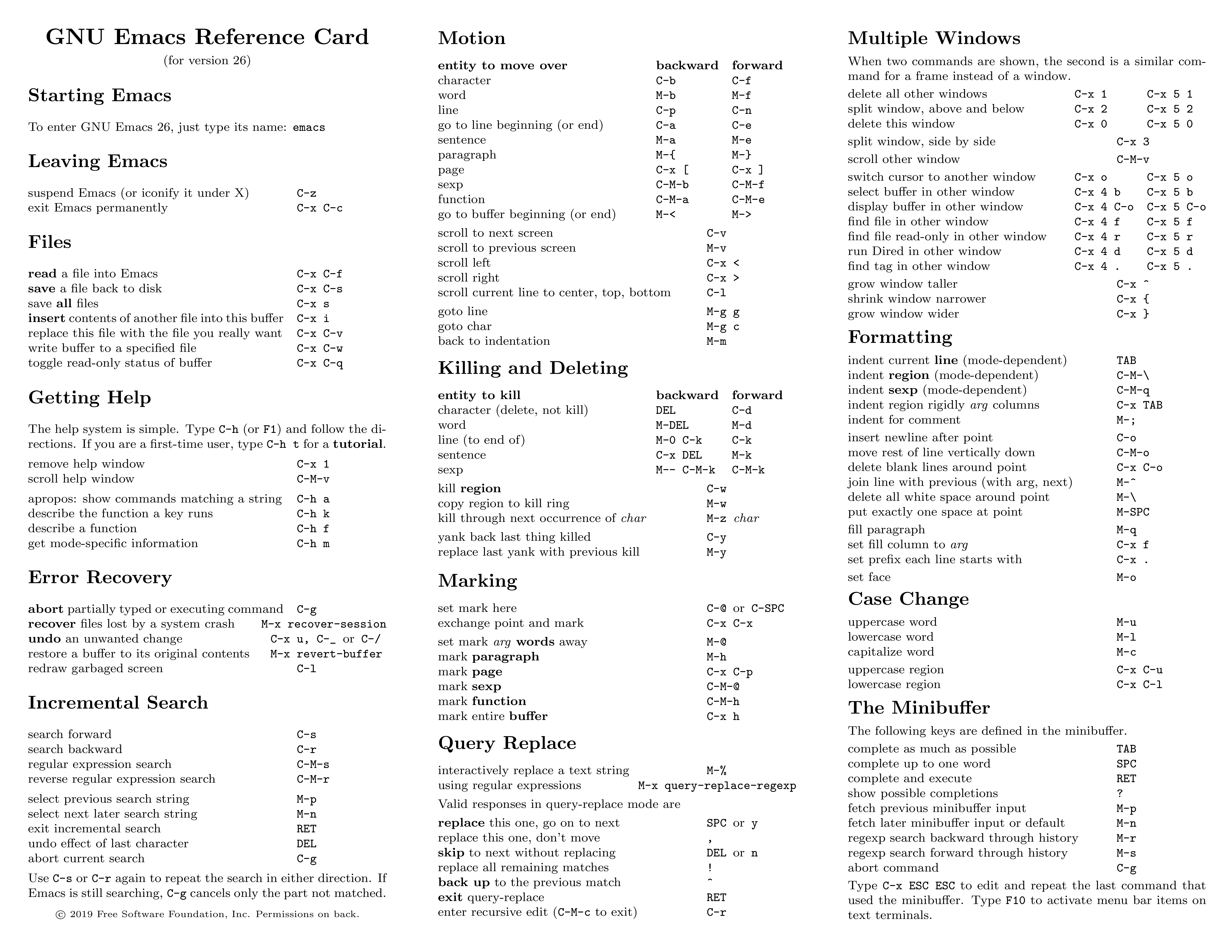
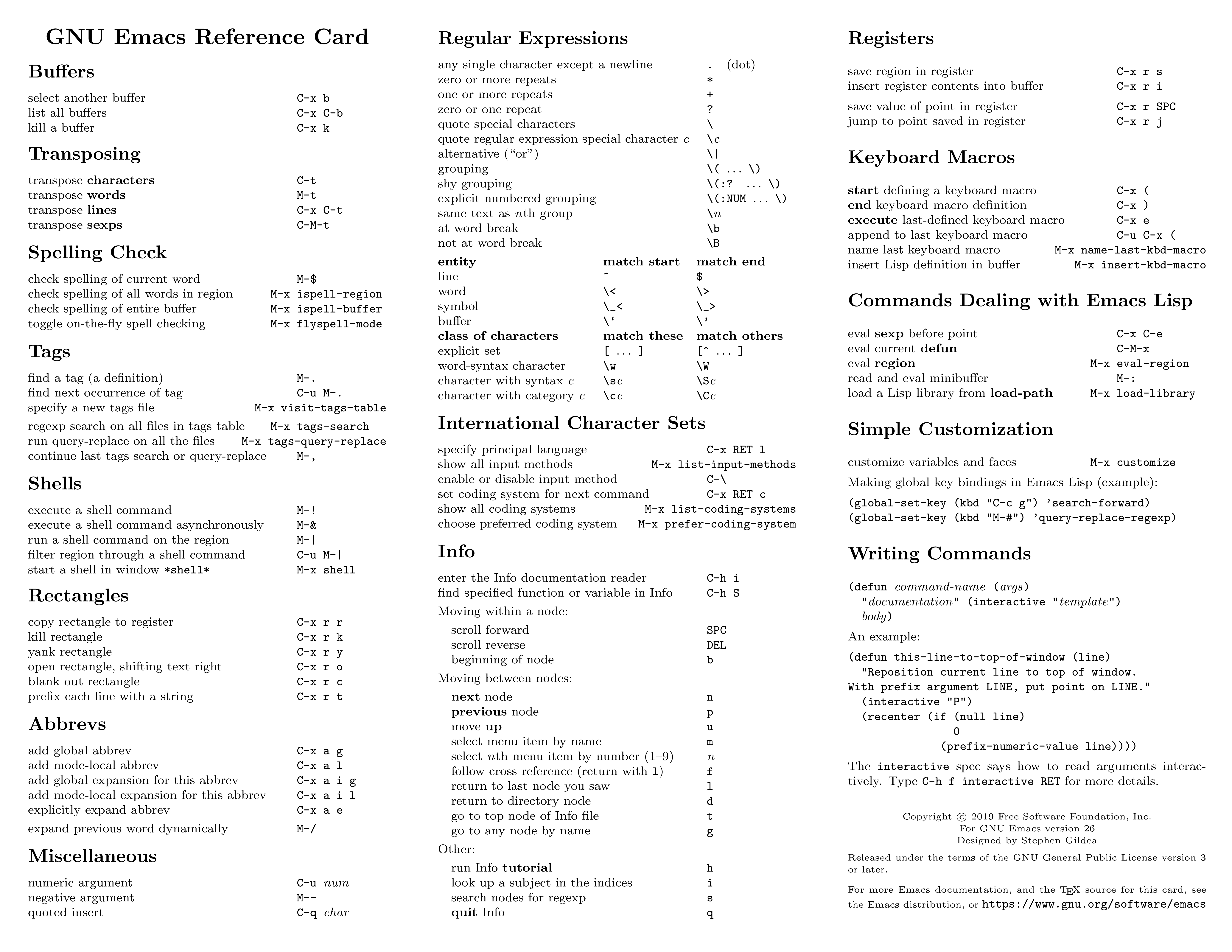
Emacs is an extensible, customizable, open-source text editor. Together with Vi/Vim is one the most widely used editors in Linux environments. There are a big number of commands, customization and extra modules that can be integrated with Emacs. We will just go briefly covering the basics.
The number of commands for Emacs is large, here the basic list of commands for editing, moving and searching text.
The best way of learning is keeping at hand a sheet of paper with the commands For example GNU Emacs Reference Card can show you most commands that you need.
Below you can see the same 2 page Reference Card as individual images.
Vi/Vim
The third editor widely supported on Linux systems is "vi". Over the years since its creation, vi became the *de-facto* standard Unix editor. The Single UNIX Specification specifies vi, so every conforming system must have it.
vi is a modal editor: it operates in either insert mode (where typed text becomes part of the document) or normal mode (where keystrokes are interpreted as commands that control the edit session). For example, typing i while in normal mode switches the editor to insert mode, but typing i again at this point places an "i" character in the document. From insert mode, pressing ESC switches the editor back to normal mode.
Vim is an improved version of the original vi, it offers
Here is a summary of the main commands used on vi. On Spruce when using "vi" you are actually using "vim".
This is very beautiful Reference Card for vim
This card was originally from this website Vim CheatSheet. The figure is very nice. However, we are not endorsing its usage by any means and I do not know about the legitimacy of the website.
Exercise
Select the editor that you know the less. The challenge is write this code in a file called Sierpinski.c
#include <stdio.h>

#define SIZE (1 << 5)
int main()
{
    int x, y, i;
    for (y = SIZE - 1; y >= 0; y--, putchar('\n')) {
        for (i = 0; i < y; i++) putchar(' ');
        for (x = 0; x + y < SIZE; x++)
            printf((x & y) ? "  " : "* ");
    }
    return 0;
}
Here is the challenge. You cannot use the arrow keys. Not a single time! It is pretty hard if you are not used to, but it is a good exercise to force you to learn the commands.
Another interesting challenge is to write the line for (y = SIZE - 1; y >= 0; y--, putchar('\n')) and copy and paste it to form the other 2 for loops in the code, and editing only after being copied.
Once you have succeed writing the source you can see your hard work in action.
On the terminal screen execute this:
$> gcc Sierpinski.c -o Sierpinski
This will compile your source code Sierpinski.c in C into a binary executable called Sierpinski. Execute the code with:
$> ./Sierpinski
The resulting output is kind of a surprise so I will not post it here. The original code comes from rosettacode.org
Why vi was programmed to not use the arrow keys?
From Wikipedia with a anecdotal story from The register
Joy used a Lear Siegler ADM-3A terminal. On this terminal, the Escape key was at the location now occupied by the Tab key on the widely used IBM PC keyboard (on the left side of the alphabetic part of the keyboard, one row above the middle row). This made it a convenient choice for switching vi modes. Also, the keys h,j,k,l served double duty as cursor movement keys and were inscribed with arrows, which is why vi uses them in that way. The ADM-3A had no other cursor keys. Joy explained that the terse, single character commands and the ability to type ahead of the display were a result of the slow 300 baud modem he used when developing the software and that he wanted to be productive when the screen was painting slower than he could think.

Key Points
Learn the basic commands to use nano, emacs and vim
The Sieve of Eratosthenes
Overview
Teaching: 45 min
Exercises: 15 minQuestions
How one algorithm looks in 7 different languages?
Objectives
Learn basic syntax from several languages used in scientific computing
Programming Languages for Scientific Computing
There are literally hundreds of programming languages. However, not all of them are suitable or commonly used for Scientific Computing. On this lesson we will present a selection of the most prominent languages for Scientific Computing today.
Without entering in subtle details, we can classify programming languages in several ways, with some shadow zones in between. Programming languages can be:
-
Interpreted or Compiled
-
Static Typed or Dynamic Typed.
In general compiled languages are also static typed and interpreted languages are dynamically typed. Examples of compiled languages are C/C++ and Fortran, in the category of interpreted we can mention Python, R and Julia. Java is an special case where code is compiled in a intermediate representation called “bytecode” that is interpreted by the Java Virtual Machine during execution.
The difference is even more diffuse by technologies like Just-in-Time compilation that uses compilation during runtime for an usually interpreted language.
There are only 3 languages that we can consider as truly High-Performance Programming Languages (PL), this trinity is made by Fortran, C and C++. Other languages, like Python and R even if used very often in Scientific Computing are not High-Performance at its core. Julia is a newer language filling the gap in this classification.
Fortran, C and C++ are all of them static typed, compiled and the most prominent paradigms for Parallel Computing in CPUs OpenMP and MPI has official support for those 3 languages. Among the list of languages that we will consider today they are also the older ones.
The next table shows the age of several languages used in Scientific Computing.
The Age of Programming Languages (by 2018)
Language First appeared Stable Release Fortran 1957; 61 years ago Fortran 2008 (ISO/IEC 1539-1:2010) / 2010; 8 years ago C 1972; 46 years ago C11 / December 2011; 6 years ago C++ 1985; 33 years ago ISO/IEC 14882:2017 / 1 December 2017; 7 months ago Python 1990; 27 years ago 3.7.0 / 27 June 2018; 2.7.15 / 1 May 2018 R 1993; 24 years ago 3.5.1 (“Feather Spray”)/ July 2, 2018 Java 1995; 23 years ago Java 10, released on March 20, 2018 Julia 2012; 6 years ago 0.6.4 / 9 July 2018
More about programming languages
The figure above was found on this Blog: Languages you should know

The Sieve of Eratosthenes
In order to illustrate all those languages in a short glimpse we will be showing how to implement the same algorithm in all those 7 languages. The algorithm is called the Sieve of Eratosthenes and it is a classical algorithm for finding all prime numbers up to any given limit. These are the rules for the implementation.
-
All implementations will be as close as possible to each other. In fact, that is a bad idea from the performance point of view but, for our purpose will facilitate the comparison in syntax rather how to achieve top performance with each PL.
-
No external libraries will be used, with the sole exception of Input/Output routines. Interpreted languages take advantage of external libraries to improve performance, those external languages are usually written in a compiled language, that is the case of several R and Python libraries.
-
The fairly accelerate the algorithm we will skip all even numbers, there is just one prime even number and we know what it is.

For this exercises, please enter in interactive mode as the head node cannot take all users executing at the same time. The Sieve was chosen for being very CPU intensive but with little memory requirements.
R
Lets start with interpreted languages. R is one of the most used languages for statistical analysis. The sieve here is implemented as an Rscript and uses a full dimension for the array. It expects one integer argument as the upper limit for the sieve, otherwise defaults to 100.
#!/usr/bin/env Rscript

SieveOfEratosthenes <- function(n) {
  if (n < 2) return(NULL)
  primes <- rep(T, n)
  sprintf(" Dimension of array %d", length(primes))

  # 1 is not prime
  primes[1] <- F
  for(i in seq(n)) {
    if (primes[i]) {
      j <- i * i
      if (j > n){
      	 if (sum(primes, na.rm=TRUE)<10000) {
	    # Select just the indices of True values
	    print(which(primes))
	 }
	 return(sum(primes, na.rm=TRUE))
	 }
      primes[seq(j, n, by=i)] <- F
    }
  }
  return()
}

# Collecting arguments from the command
args = commandArgs(trailingOnly=TRUE)

# Default number is n=100
if (length(args)==0) {
  n = 100
} else {
  n = strtoi(args[1])
}

sprintf(" Prime numbers up to %d", n)
nprimes<-SieveOfEratosthenes(n)
sprintf(" Total number of primes found: %d", nprimes)
Now lets get some timing on how much it takes for the first 100 million integers. This timing was taking on Spruce but your numbers could be different based on which compute node are you running.
$ time ./SieveOfEratosthenes.R 100000000
[1] " Prime numbers up to 100000000"
[1] " Total number of primes found: 5761455"

real    0m24.492s
user    0m23.672s
sys     0m0.823s
Exercise: Writing the code with a text editor
Using the editor of your choice (nano for example), write the code above and store it in a file.
Create a folder and move the file into that folder.
Execute the code as show above for less than 100 thousand integers. For larger values a submission script must be used and we will see that on our next episode.
Key Points
A literal translation of an algorithm ends up in a poorly efficient code.
Each language has its own way of doing things. Knowing how to adapt the algorithm to the language is the way to create efficient code.
Job Submission (Torque and Moab)
Overview
Teaching: 30 min
Exercises: 30 minQuestions
How to submit jobs on the HPC cluster?
Objectives
Learn the most frequently used commands for Torque and Moab
When you are using your own computer, you execute your calculations and you are responsible of not overloading the machine with more workload that the machine can actually process efficiently. Also, you probably have only one machine to work, if you have several you login individually on each and execute calculations by directly running calculations.
On a shared resource like an HPC cluster, things are very different. You and several others, maybe hundreds are competing for getting their calculations done. A Resource Manager take care of receiving job submissions. From the other side a Job Scheduler is in charge of associate jobs with the appropriated resources and trying to maximize and objective function such as total utilization constrained by priorities and the best balance between the resources requested and resources available.
TORQUE Resource and Queue Manager
Terascale Open-source Resource and QUEue Manager (TORQUE) is a distributed resource manager providing control over batch jobs and distributed compute nodes. TORQUE can be integrated both, commercial and non-commercial Schedulers. In the case of Mountaineer and Spruce TORQUE is used with the commercial Moab Scheduler.
This is a list of TORQUE commands:
| Command | Description |
|---|---|
momctl |
Manage/diagnose MOM (node execution) daemon |
pbsdsh |
Launch tasks within a parallel job |
pbsnodes |
View/modify batch status of compute nodes |
qalter |
Modify queued batch jobs |
qchkpt |
Checkpoint batch jobs |
qdel |
Delete/cancel batch jobs |
qgpumode |
Specifies new mode for GPU |
qgpureset |
Reset the GPU |
qhold |
Hold batch jobs |
qmgr |
Manage policies and other batch configuration |
qmove |
Move batch jobs |
qorder |
Exchange order of two batch jobs in any queue |
qrerun |
Rerun a batch job |
qrls |
Release batch job holds |
qrun |
Start a batch job |
qsig |
Send a signal to a batch job |
qstat |
View queues and jobs |
qsub |
Submit jobs |
qterm |
Shutdown pbs server daemon |
tracejob |
Trace job actions and states recorded in Torque logs (see Using “tracejob” to Locate Job Failures) |
From those commands, a basic knowledge about qsub, qstat and qdel is suficient for most purposes on a normal usage of the cluster.
TORQUE includes numerous directives, which are used to specify resource
requirements and other attributes for batch and interactive jobs.
TORQUE directives can appear as header lines (lines that start with #PBS)
in a batch job script or as command-line options to the qsub command.
Submission scripts
A TORQUE job script for a serial job might look like this:
#!/bin/bash
#PBS -k o
#PBS -l nodes=1:ppn=1,walltime=00:30:00
#PBS -M username@mix.wvu.edu
#PBS -m abe
#PBS -N JobName
#PBS -j oe
#PBS -q standby

cd $PBS_O_WORKDIR
./a.out
The following table describes the most basic directives
| TORQUE directive | Description |
|---|---|
| #PBS -k o | Keeps the job output |
| #PBS -l nodes=1:ppn=1,walltime=00:30:00 | Indicates the job requires one node, one processor per node, and 30 minutes of wall-clock time |
| #PBS -M username@mix.wvu.edu | Sends job-related email to username@mix.wvu.edu |
| #PBS -m abe | Sends email if the job is (a) aborted, when it (b) begins, and when it (e) ends |
| #PBS -N JobName | Names the job JobName |
| #PBS -j oe | Joins standard output and standard error |
| #PBS -q standby | Submit the job on the standby queue |
A parallel job using MPI could be like this:
#!/bin/bash
#PBS -k o
#PBS -l nodes=1:ppn=16,walltime=30:00
#PBS -M username@mix.wvu.edu
#PBS -m abe
#PBS -N JobName
#PBS -j oe
#PBS -q standby

cd $PBS_O_WORKDIR
mpirun -np 16 -machinefile $PBS_NODEFILE ./a.out
The directives are very similar to the serial case
| TORQUE directive | Description |
|---|---|
| #PBS -l nodes=1:ppn=16,walltime=00:30:00 | Indicates the job requires one node, using 16 processors per node, and 30 minutes of runtime. |
Exercise: Creating a Job script and submit it
On
1.Intro-HPC/07.jobsyou will find the same 3 ABINIT files that we worked on the Command Line Interface episode. The exercise is to prepare a submission script for computing the calculation. This is all that you need to know:
- You need to load the these modules to use ABINIT
module load compilers/gcc/6.3.0 mpi/openmpi/2.1.2_gcc63 libraries/fftw/3.3.6_gcc63 compilers/intel/17.0.1_MKL_only atomistic/abinit/8.6.3_gcc63It is good idea to purge the modules first to avoid conflicts with the modules that you probably are loading by default.
- ABINIT works in parallel using MPI, for this exercise lets request 4 cores on a single node. The actual command to be executed is:
mpirun -np 4 abinit < t17.filesAssuming that you have moved into the folder that has the 3 files.
Job Arrays
Job array is a way to submit many jobs that can be indexed. The jobs are independent between them but you can submit them with a single qsub
#!/bin/sh

#PBS -N <jobname>_${PBS_ARRAYID}
#PBS -t <num_range>
#PBS -l nodes=<number_of_nodes>:ppn=<PPN number>,walltime=<time_needed_by_job>
#PBS -m ae
#PBS -M <email_address>
#PBS -q <queue_name>
#PBS -j oe

cd $PBS_O_WORKDIR
# Enter the command here
mpirun -np <PPN number> ./a.out
There a few new elements here: ${PBS_ARRAYID} is a variable that receives one different value for each job in the range described from the -t variable.
#PBS -j oe is an option often used for job arrays, it merges the standard output and error files in a single file, avoiding the overload of files for large job arrays.
Exercise: Job arrays
Using the same 3 files from our previous exercise, prepare a set of 5 folders called
1,2,3,4and5. The file14si.pspncis better as a symbolic link as that file will never change.Solution
 $ mkdir 1 2 3 4 5
 $ cp t17.* 1
 $ cp t17.* 2
 $ cp t17.* 3
 $ cp t17.* 4
 $ cp t17.* 5
 $ ln -s ../14si.pspnc 1/14si.pspnc
 $ ln -s ../14si.pspnc 2/14si.pspnc
 $ ln -s ../14si.pspnc 3/14si.pspnc
 $ ln -s ../14si.pspnc 4/14si.pspnc
 $ ln -s ../14si.pspnc 5/14si.pspnc
Modify the submission script from the previous exercise to create a job array. When executed, each job in the array receives a different value inside
${PBS_ARRAYID}, we use the value to go into the corresponding folder and execute ABINIT there.solution
#!/bin/bash

#PBS -N ABINIT_${PBS_ARRAYID}
#PBS -l nodes=1:ppn=4
#PBS -q debug
#PBS -t 1-5
#PBS -j oe

module purge
module load compilers/gcc/6.3.0 mpi/openmpi/2.1.2_gcc63 libraries/fftw/3.3.6_gcc63 compilers/intel/17.0.1_MKL_only  atomistic/abinit/8.6.3_gcc63

cd $PBS_O_WORKDIR
cd ${PBS_ARRAYID}

mpirun -np 4 abinit < t17.files
Environment variables
We are using PBS_O_WORKDIR to change directory to the place where the job was submitted The following environment variables will be available to the batch job.
| Variable | Description |
|---|---|
| PBS_O_HOST | the name of the host upon which the qsub command is running. |
| PBS_SERVER | the hostname of the pbs_server which qsub submits the job to. |
| PBS_O_QUEUE | the name of the original queue to which the job was submitted. |
| PBS_O_WORKDIR | the absolute path of the current working directory of the qsub command. |
| PBS_ARRAYID | each member of a job array is assigned a unique identifier (see -t) |
| PBS_ENVIRONMENT | if set to PBS_BATCH is a batch job, if set to PBS_INTERACTIVE is an interactive job. |
| PBS_JOBID | the job identifier assigned to the job by the batch system. |
| PBS_JOBNAME | the job name supplied by the user. |
| PBS_NODEFILE | the name of the file contain the list of nodes assigned to the job (for parallel and cluster systems). |
| PBS_QUEUE | the name of the queue from which the job is executed. |
Montioring jobs
To monitor the status of a queued or running job, use the qstat command from Torque of showq from Moab.
Useful qstat options include:
| qstat option | Description |
|---|---|
| -Q | show all queues available |
| -u user_list | Displays jobs for users listed in user_list |
| -a | Displays all jobs |
| -r | Displays running jobs |
| -f | Displays the full listing of jobs (returns excessive detail) |
| -n | Displays nodes allocated to jobs |
Moab showq offers:
| showq option | Description |
|---|---|
| -b | blocked jobs only |
| -c | details about recently completed jobs. |
| -g | grid job and system id’s for all jobs. |
| -i | extended details about idle jobs. |
| -l | local/remote view. For use in a Grid environment, displays job usage of both local and remote compute resources. |
| -n | normal showq output, but lists job names under JOBID |
| -o | jobs in the active queue in the order specified (uses format showq -o |
| -p | only jobs assigned to the specified partition. |
| -r | extended details about active (running) jobs. |
| -R | only jobs which overlap the specified reservation. |
| -u | specified user’s jobs. Use showq -u -v to display the full username if it is truncated in normal -u output. |
| -v | local and full resource manager job IDs as well as partitions. |
| -w | only jobs associated with the specified constraint. Valid constraints include user, group, acct, class, and qos. |
Deleting jobs
With Torque you can use qdel. Moab uses mjobctl -c. For example:
$ qdel 1045
$ mjobctl -c 1045
Prologue and Epilogue
Torque provides administrators the ability to run scripts before and/or after each job executes. With such a script, you can prepare the system, perform node health checks, prepend and append text to output and error log files, cleanup systems, and so forth.
You can add prologue and epilogue scripts from the command line.
$ qsub -l prologue=/home/user/prologue.sh,epilogue=/home/user/epilogue.sh
or adding the corresponding lines on your submission script.
#!/bin/bash
...
#PBS -l prologue=/home/user/prologue.sh
#PBS -l
...
A simple prologue.sh can be like this:
#!/bin/sh

echo "Prologue Args:"
echo "Job ID: $1"
echo "User ID: $2"
echo "Group ID: $3"
echo ""

exit 0
And a simple epilogue can be like:
#!/bin/sh

echo "Epilogue Args:"
echo "Job ID: $1"
echo "User ID: $2"
echo "Group ID: $3"
echo "Job Name: $4"
echo "Session ID: $5"
echo "Resource List: $6"
echo "Resources Used: $7"
echo "Queue Name: $8"
echo "Account String: $9"
echo ""

exit 0
The purpose of the scripts above is to provide information about the job being stored in the same file as the standard output file created for the job. That is very useful if you want to adjust resources based on previous executions and the epilogue will store the information on file.
The prologue is also useful, it can check if the proper environment for the job is present and based on the return of that script indicate Torque if the job should continue for execution, resubmit it or cancel it. The following table describes each exit code for the prologue scripts and the action taken.
| Error | Description | Action |
|---|---|---|
| -4 | The script timed out | Job will be requeued |
| -3 | The wait(2) call returned an error | Job will be requeued |
| -2 | Input file could not be opened | Job will be requeued |
| -1 | Permission error (script is not owned by root, or is writable by others) | Job will be requeued |
| 0 | Successful completion | Job will run |
| 1 | Abort exit code | Job will be aborted |
| >1 | other | Job will be requeued |
Exercise: Prologue and Epilogue arrays
Add prologue and epilogue to the job array from the previous exercise
Interactive jobs with X11 Forwarding
Sometimes you need to do some interactive job to create some plots and we would like to see the figures on the fly rather than, bring all the data back to the desktop, this example shows how to achieve that.
$ ssh -Y username@spruce.hpc.wvu.edu
Test the X11 Forwarding
$ xeyes
A windows should appear with two eyes facing you, you can close the window and create a new session with qsub
$ qsub -X -I
After you get a new session and test it again with xeyes. This new eyes comes from the compute node, not from the head node.
$ xeyes
Lets suppose that the plot will be created with R, load the module for R 3.4.1 (the latest version by the time this was written)
$ module load compilers/R/3.4.1
Enter in the text-based R interpreter
$ R
Test a simple plot in R
> # Define the cars vector with 5 values
> cars <- c(1, 3, 6, 4, 9)
>

> # Graph the cars vector with all defaults
> plot(cars)
>
You should get a new window with a plot and a few points. On the episode about Singularity we will see some other packages that use the X11 server like RStudio and Visit.
Key Points
It is a good idea to keep aliases to common torque commands for easy execution.