Overview

Teaching: 45 min
Exercises: 15 min

Questions

• How one algorithm looks in 7 different languages?

Objectives

• Learn basic syntax from several languages used in scientific computing

Programming Languages for Scientific Computing

There are literally hundreds of programming languages. However, not all of them are suitable or commonly used for Scientific Computing. On this lesson we will present a selection of the most prominent languages for Scientific Computing today.

Without entering in subtle details, we can classify programming languages in several ways, with some shadow zones in between. Programming languages can be:

1. Interpreted or Compiled

2. Static Typed or Dynamic Typed.

In general compiled languages are also static typed and interpreted languages are dynamically typed. Examples of compiled languages are C/C++ and Fortran, in the category of interpreted we can mention Python, R and Julia. Java is an special case where code is compiled in a intermediate representation called “bytecode” that is interpreted by the Java Virtual Machine during execution.

The difference is even more diffuse by technologies like Just-in-Time compilation that uses compilation during runtime for an usually interpreted language.

There are only 3 languages that we can consider as truly High-Performance Programming Languages (PL), this trinity is made by Fortran, C and C++. Other languages, like Python and R even if used very often in Scientific Computing are not High-Performance at its core. Julia is a newer language filling the gap in this classification.

Fortran, C and C++ are all of them static typed, compiled and the most prominent paradigms for Parallel Computing in CPUs OpenMP and MPI has official support for those 3 languages. Among the list of languages that we will consider today they are also the older ones.

The next table shows the age of several languages used in Scientific Computing.

The Age of Programming Languages (by 2018)

Language	First appeared	Stable Release
Fortran	1957; 61 years ago	Fortran 2008 (ISO/IEC 1539-1:2010) / 2010; 8 years ago
C	1972; 46 years ago	C11 / December 2011; 6 years ago
C++	1985; 33 years ago	ISO/IEC 14882:2017 / 1 December 2017; 7 months ago
Python	1990; 27 years ago	3.7.0 / 27 June 2018; 2.7.15 / 1 May 2018
R	1993; 24 years ago	3.5.1 (“Feather Spray”)/ July 2, 2018
Java	1995; 23 years ago	Java 10, released on March 20, 2018
Julia	2012; 6 years ago	0.6.4 / 9 July 2018

More about programming languages

The figure above was found on this Blog: Languages you should know

The Sieve of Eratosthenes

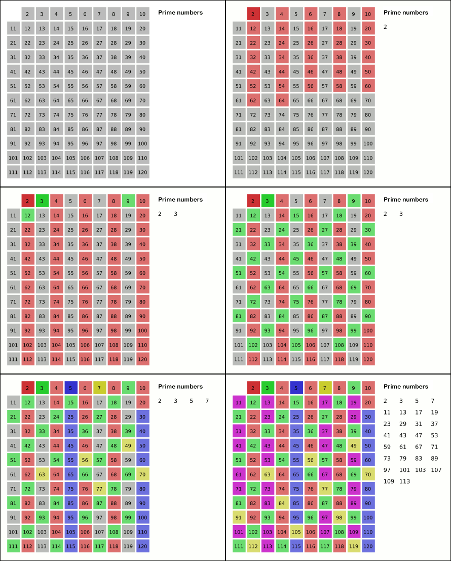
In order to illustrate all those languages in a short glimpse we will be showing how to implement the same algorithm in all those 7 languages. The algorithm is called the Sieve of Eratosthenes and it is a classical algorithm for finding all prime numbers up to any given limit. These are the rules for the implementation.

1. All implementations will be as close as possible to each other. In fact, that is a bad idea from the performance point of view but, for our purpose will facilitate the comparison in syntax rather how to achieve top performance with each PL.

2. No external libraries will be used, with the sole exception of Input/Output routines. Interpreted languages take advantage of external libraries to improve performance, those external languages are usually written in a compiled language, that is the case of several R and Python libraries.

3. The fairly accelerate the algorithm we will skip all even numbers, there is just one prime even number and we know what it is.

For this exercises, please enter in interactive mode as the head node cannot take all users executing at the same time. The Sieve was chosen for being very CPU intensive but with little memory requirements.

R

Lets start with interpreted languages. R is one of the most used languages for statistical analysis. The sieve here is implemented as an Rscript and uses a full dimension for the array. It expects one integer argument as the upper limit for the sieve, otherwise defaults to 100.

#!/usr/bin/env Rscript

SieveOfEratosthenes <- function(n) {
  if (n < 2) return(NULL)
  primes <- rep(T, n)
  sprintf(" Dimension of array %d", length(primes))

  # 1 is not prime
  primes[1] <- F
  for(i in seq(n)) {
    if (primes[i]) {
      j <- i * i
      if (j > n){
      	 if (sum(primes, na.rm=TRUE)<10000) {
	    # Select just the indices of True values
	    print(which(primes))
	 }  
	 return(sum(primes, na.rm=TRUE))
	 }	 
      primes[seq(j, n, by=i)] <- F
    }
  }
  return()
}

# Collecting arguments from the command
args = commandArgs(trailingOnly=TRUE)

# Default number is n=100
if (length(args)==0) {
  n = 100
} else {
  n = strtoi(args[1])
}

sprintf(" Prime numbers up to %d", n)
nprimes<-SieveOfEratosthenes(n)
sprintf(" Total number of primes found: %d", nprimes)

Now lets get some timing on how much it takes for the first 100 million integers. This timing was taking on Spruce but your numbers could be different based on which compute node are you running.

$ time ./SieveOfEratosthenes.R 100000000

[1] " Prime numbers up to 100000000"
[1] " Total number of primes found: 5761455"

real    0m24.492s
user    0m23.672s
sys     0m0.823s

Exercise: Writing the code with a text editor

• Using the editor of your choice (nano for example), write the code above and store it in a file.

• Create a folder and move the file into that folder.

• Execute the code as show above for less than 100 thousand integers. For larger values a submission script must be used and we will see that on our next episode.

Key Points

• A literal translation of an algorithm ends up in a poorly efficient code.

• Each language has its own way of doing things. Knowing how to adapt the algorithm to the language is the way to create efficient code.