Introduction to GPU Computing
Overview
Teaching: 30 min
Exercises: 0 minQuestions
What is GPU?
How a GPU is different from a CPU?
Which scientific problems work better on GPUs?
Objectives
Learn about how and why GPUs are important today in scientific computing
Understand the differences and similarities of GPUs and CPUs for scientific computing
Heterogeneous Parallel Computing
For basically all the 21st century two trends have dominated the area of High Perfomance Computing. The first one is the increase number of cores in CPUs from the dual core to the current CPUs on consumer market with 4, 8 and more cores. The second trend is the availability of modern coprocessors.
Coprocessors are devices that take some processing out of the CPU by specializing on specific tasks. Those coprocessors have not all the capabilities of CPUs and in general are not able to act as a CPU but they are very efficient in certain tasks. Examples of coprocessors in recent years are the Intel Xeon Phi coprocessors and most notoriously for this lesson GPUs in particular those from NVIDIA that thanks to CUDA we will examine in these series of lectures.
These trends will most likely follow and enhance in the foreseeable future. CPUs will come with 20, 40 and even more cores per socket. GPUs will become more common in addition to another specialized coprocessors such as FPGAs, and neural processors.
In this lesson we will concentrate on parallel computing with CUDA and OpenACC. The central theme about using GPUs is to manage a large number of computing threads a number that is 2 or 3 orders of magnitude larger than the number of computing threads on CPUs. In contrast to what is called multithreading parallel computing, on GPUs we talk about many-threading parallel computing.
The first GPUs used for general computing, came from repurposing GPUs. GPUs were originally designed to compute textures, graphics and rotations of 3D graphics for display on screen. These tasks do not require for most part double precision numbers. Only relatively recently double precision capabilities were integrated in those GPUs but for most part significant performance edge can be achieved when you can work with single precision floats.
Memory bandwidth is another important constrainer in GPUs. As GPUs have their own memory and cannot manage the central RAM, the ability to perform better on a GPU depends on enough processing being done with the data allocated on the GPU memory before the data is copied back to the Host RAM. A GPU must be capable of transferring large amounts of data, processing the data for a meaningful mount of time and return the results back in order to produce a positive return.
As such GPUs were designed for very specific tasks and not all tasks can be efficiently being offloaded to the GPU. There are tasks for which CPUs perform better and will continue to do so in the near future. At the end we will have what we called heterogeneous parallel computing a paradigm where parallel computing is exploited at 3 different and even entangled levels.
First is CPU multithreading execution. In the next lesson we will demonstrate one example of OpenMP a popular model for these kind of parallelism. In CPU multithreading we use the ability of modern CPUs to have several cores that see the same memory. The next level is coprocessor parallelism, exemplified with OpenACC, OpenCL and CUDA. Using for example GPUs certain tasks what require many threads with relatively small amount of memory can be processed on those devices and get an advantage from them. The final level is distributed computing with a prototypical case is MPI. We will demonstrate a brief example of MPI in the next lesson but it is out of scope for this workshop.
Accelerators (like GPUs) in the world largest supercomputers
NVIDIA GPUs Powered 168 of The Top500 Supercomputers On The Planet. Eight of the world’s top 10 supercomputers now use NVIDIA GPUs, InfiniBand networking or both. They include the most powerful systems in the U.S., Europe and China. The fastest supercomputers all rely on Accelerators. More than 50% of the computational power in the top500 comes from accelerators.
As per the latest figures, it looks like NVIDIA GPUs are powering the bulk of the supercomputers in the Top500 list with a total of 168 systems while AMD’s CPUs and GPUs power a total of 121 supercomputers. At the same time, Supercomputers housing AMD and NVIDIA GPU-based accelerators are largely running Intel CPUs which cover around 400 supercomputers and that’s a huge figure & while the number of systems running Intel CPUs are in a clear lead in quantity, AMD actually wins the crown for the fastest supercomputer around in the form of Frontier.
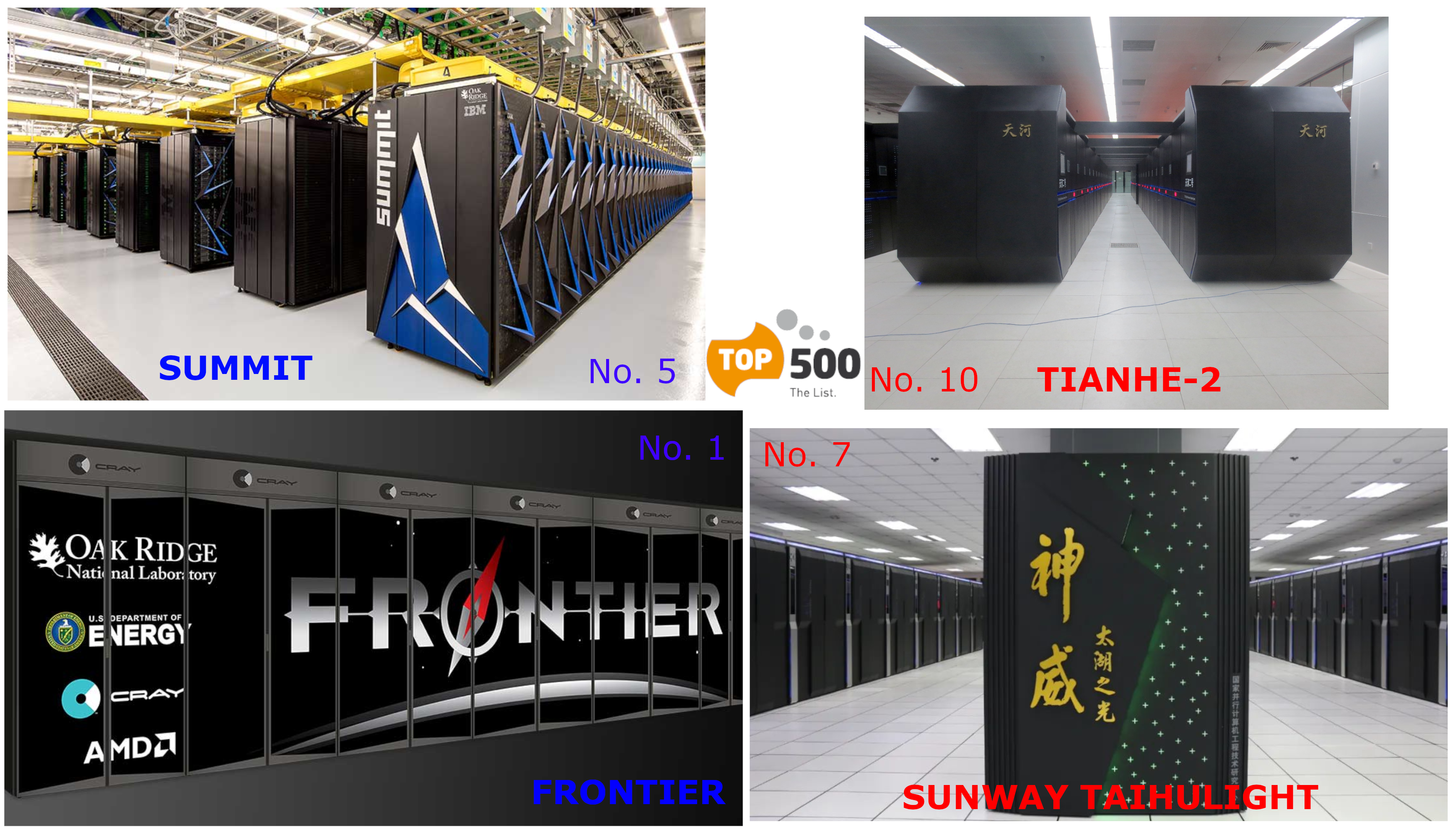
Frontier
HPE Cray EX235a, AMD Optimized 3rd Generation EPYC 64C 2GHz, AMD Instinct MI250X, Slingshot-11, HPE DOE/SC/Oak Ridge National Laboratory United States
- CPU cores 8,699,904
- Rmax (PFlop/s): 1,194.00
- Rpeak (PFlop/s) : 1,679.82
- Power (kW) : 22,703
Summit
IBM Power System AC922, IBM POWER9 22C 3.07GHz, NVIDIA Volta GV100, Dual-rail Mellanox EDR Infiniband, IBM DOE/SC/Oak Ridge National Laboratory United States
- CPU cores 2,414,592
- Rmax (PFlop/s): 148.60
- Rpeak (PFlop/s) : 200.79
- Power (kW) : 10,096
WVU High-Performance Computer Clusters
West Virginia University has 2 main clusters: Thorny Flat and Dolly Sods, our newest cluster that will be available later in August 2023.
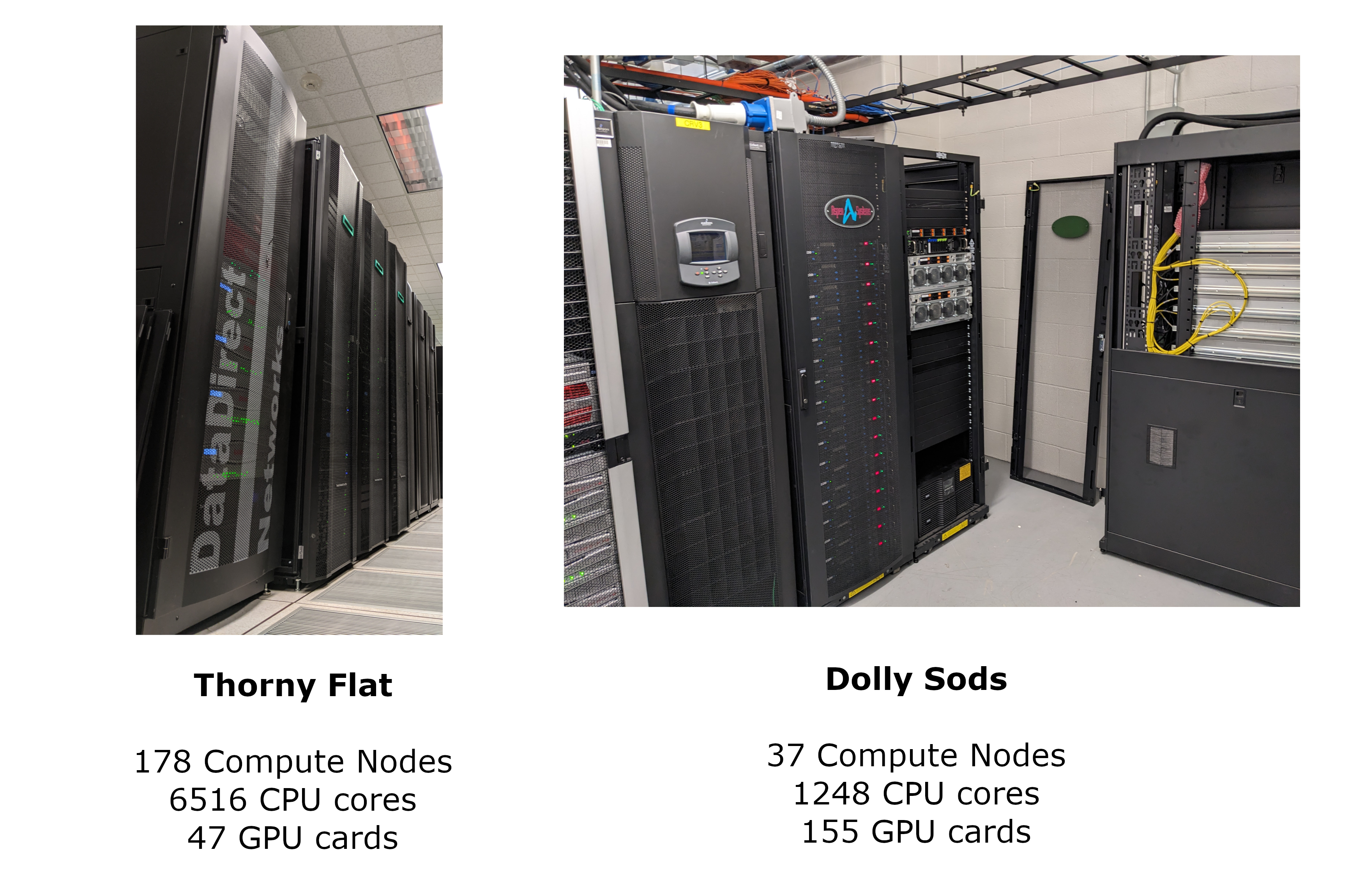
Thorny Flat
Thorny Flat is a general-purpose HPC cluster with 178 compute nodes, most nodes have 40 CPU cores. The total CPU core count is 6516 cores. There are 47 NVIDIA GPU cards ranging from P6000, RTX6000, and A100
Dolly Sods
Dolly Sods is our newest cluster and it is specialized in GPU computing. It has 37 nodes and 155 NVIDIA GPU cards ranging from A30, A40 and A100. The total CPU core count is 1248.
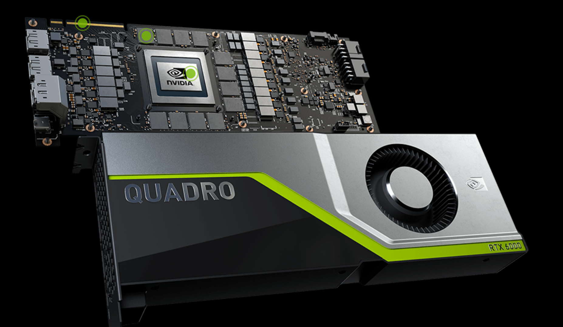
GPUs on Thorny Flat
NVIDIA Quadro RTX6000
| RTX 6000 | P 6000 | |
|---|---|---|
| Architecture | Turing | Pascal |
| CUDA Parallel-Processing Cores | 4,608 | 3,840 |
| Bus width | 384 bit | 384 bit |
| Memory Clock | 1750 | 1127 MHz |
| NVIDIA Tensor Cores | 576 | |
| NVIDIA RT Cores | 72 | |
| GPU Memory | 24 GB GDDR6 | 24 GB GDDR5X |
| FP32 Performance | 16.3 TFLOPS | 12.63 TFLOPS |
| FP64 Performance | 564 GFLOPS | 394 GFLOPS |
| Max Power Consumption | 260 W | 250 W |
| CUDA | 6.1 | 6.1 |
| OpenCL | 1.2 | 1.2 |
Knowing the GPUs on the machine
A first view of the availability of GPUs can be seen with the command:
$> nvidia-smi
Thorny Flat has several machines with GPUs the output in one of them is:
+-----------------------------------------------------------------------------+
| NVIDIA-SMI 455.32.00    Driver Version: 455.32.00    CUDA Version: 11.1     |
|-------------------------------+----------------------+----------------------+
| GPU  Name        Persistence-M| Bus-Id        Disp.A | Volatile Uncorr. ECC |
| Fan  Temp  Perf  Pwr:Usage/Cap|         Memory-Usage | GPU-Util  Compute M. |
|                               |                      |               MIG M. |
|===============================+======================+======================|
|   0  Quadro P6000        Off  | 00000000:37:00.0 Off |                  Off |
| 16%   28C    P0    58W / 250W |      0MiB / 24449MiB |      0%   E. Process |
|                               |                      |                  N/A |
+-------------------------------+----------------------+----------------------+
|   1  Quadro P6000        Off  | 00000000:AF:00.0 Off |                  Off |
| 17%   27C    P0    57W / 250W |      0MiB / 24449MiB |      0%   E. Process |
|                               |                      |                  N/A |
+-------------------------------+----------------------+----------------------+
|   2  Quadro P6000        Off  | 00000000:D8:00.0 Off |                  Off |
| 16%   28C    P0    58W / 250W |      0MiB / 24449MiB |      0%   E. Process |
|                               |                      |                  N/A |
+-------------------------------+----------------------+----------------------+

+-----------------------------------------------------------------------------+
| Processes:                                                                  |
|  GPU   GI   CI        PID   Type   Process name                  GPU Memory |
|        ID   ID                                                   Usage      |
|=============================================================================|
|  No running processes found                                                 |
+-----------------------------------------------------------------------------+
+-----------------------------------------------------------------------------+
| NVIDIA-SMI 455.32.00    Driver Version: 455.32.00    CUDA Version: 11.1     |
|-------------------------------+----------------------+----------------------+
| GPU  Name        Persistence-M| Bus-Id        Disp.A | Volatile Uncorr. ECC |
| Fan  Temp  Perf  Pwr:Usage/Cap|         Memory-Usage | GPU-Util  Compute M. |
|                               |                      |               MIG M. |
|===============================+======================+======================|
|   0  Quadro RTX 6000     Off  | 00000000:1A:00.0 Off |                    0 |
| N/A   38C    P0    55W / 250W |      0MiB / 22698MiB |      0%      Default |
|                               |                      |                  N/A |
+-------------------------------+----------------------+----------------------+
|   1  Quadro RTX 6000     Off  | 00000000:1B:00.0 Off |                    0 |
| N/A   39C    P0    56W / 250W |      0MiB / 22698MiB |      0%      Default |
|                               |                      |                  N/A |
+-------------------------------+----------------------+----------------------+
|   2  Quadro RTX 6000     Off  | 00000000:3D:00.0 Off |                    0 |
| N/A   39C    P0    57W / 250W |      0MiB / 22698MiB |      0%      Default |
|                               |                      |                  N/A |
+-------------------------------+----------------------+----------------------+
|   3  Quadro RTX 6000     Off  | 00000000:3E:00.0 Off |                    0 |
| N/A   40C    P0    57W / 250W |      0MiB / 22698MiB |      0%      Default |
|                               |                      |                  N/A |
+-------------------------------+----------------------+----------------------+
|   4  Quadro RTX 6000     Off  | 00000000:8B:00.0 Off |                    0 |
| N/A   37C    P0    56W / 250W |      0MiB / 22698MiB |      0%      Default |
|                               |                      |                  N/A |
+-------------------------------+----------------------+----------------------+
|   5  Quadro RTX 6000     Off  | 00000000:8C:00.0 Off |                    0 |
| N/A   37C    P0    56W / 250W |      0MiB / 22698MiB |      0%      Default |
|                               |                      |                  N/A |
+-------------------------------+----------------------+----------------------+
|   6  Quadro RTX 6000     Off  | 00000000:B5:00.0 Off |                    0 |
| N/A   37C    P0    54W / 250W |      0MiB / 22698MiB |      0%      Default |
|                               |                      |                  N/A |
+-------------------------------+----------------------+----------------------+
|   7  Quadro RTX 6000     Off  | 00000000:B6:00.0 Off |                    0 |
| N/A   37C    P0    57W / 250W |      0MiB / 22698MiB |      0%      Default |
|                               |                      |                  N/A |
+-------------------------------+----------------------+----------------------+

+-----------------------------------------------------------------------------+
| Processes:                                                                  |
|  GPU   GI   CI        PID   Type   Process name                  GPU Memory |
|        ID   ID                                                   Usage      |
|=============================================================================|
|  No running processes found                                                 |
+-----------------------------------------------------------------------------+
Launching interactive sessions with GPUs
A very simple way of launching an interactive job is using the command srun:
The following is an example of a request for an interactive job asking for 1 GPU 8 CPU cores for 2 hours:
trcis001:~$ srun -p comm_gpu_inter -G 1 -t 2:00:00 -c 8 --pty bash
You can verify the assigned GPU using the command nvidia-smi:
trcis001:~$ srun -p comm_gpu_inter -G 1 -t 2:00:00 -c 8 --pty bash
srun: job 22599 queued and waiting for resources
srun: job 22599 has been allocated resources
tbegq200:~$ nvidia-smi
Wed Jan 18 13:27:01 2023
+-----------------------------------------------------------------------------+
| NVIDIA-SMI 515.43.04    Driver Version: 515.43.04    CUDA Version: 11.7     |
|-------------------------------+----------------------+----------------------+
| GPU  Name        Persistence-M| Bus-Id        Disp.A | Volatile Uncorr. ECC |
| Fan  Temp  Perf  Pwr:Usage/Cap|         Memory-Usage | GPU-Util  Compute M. |
|                               |                      |               MIG M. |
|===============================+======================+======================|
|   0  NVIDIA A100-PCI...  Off  | 00000000:3B:00.0 Off |                    0 |
| N/A   28C    P0    31W / 250W |      0MiB / 40960MiB |      0%      Default |
|                               |                      |             Disabled |
+-------------------------------+----------------------+----------------------+

+-----------------------------------------------------------------------------+
| Processes:                                                                  |
|  GPU   GI   CI        PID   Type   Process name                  GPU Memory |
|        ID   ID                                                   Usage      |
|=============================================================================|
|  No running processes found                                                 |
+-----------------------------------------------------------------------------+
The command above shows an NVIDIA A100 as the GPU assigned to us during the lifetime of the job.
Key Points
On the largest Supercomputers in the world, most of the computational power comes from accelerators such as GPUs
Not everything a CPU can do a GPU can do.
GPUs are particularly good on a restricted set of tasks
Paradigms of Parallel Computing
Overview
Teaching: 30 min
Exercises: 0 minQuestions
Which are the ways we can use parallel computing?
On which of them GPUs can be used?
Objectives
Review one example of a code written with several methods of parallelization
We will pursue an exploration of several paradigms in parallel computing, from purely CPU computing to GPU computing. The paradigms chosen were OpenMP, OpenACC, OpenCL, MPI, and CUDA. By using the same problem as baseline we hope to give a sense of perspective of how those different alternatives of parallelization work in practice.
We will be solving a very simple problem. The DAXPY function is the name given in BLAS to a routine that implements the function Y = A * X + Y where X and Y may be either native double-precision valued matrices or numeric vectors, and A is a scalar. We will be computing a trigonometric identity using DAXPY as the function that will be the target of parallelization.
We will compute this formula:
[cos(2x) = cos^2(x)-sin^2(x)]
For an array of vectors in a domain in the range of \(x=[0:\pi]\)
All the codes in this lesson will be compiled with the NVIDIA HPC compilers. That will give us some uniformity on the compiler choice as this compiler supports several of the parallel models that will be demonstrated.
To access the compilers on Thorny you need to load the module:
$> module load lang/nvidia/nvhpc/23.3
To check that the compiler is available execute:
$> nvc --version
You should get something like:
nvc 23.3-0 64-bit target on x86-64 Linux -tp skylake-avx512
NVIDIA Compilers and Tools
Copyright (c) 2022, NVIDIA CORPORATION & AFFILIATES.  All rights reserved.
Serial Code
We will start without parallelization. The term given to codes that use one single sequence of instructions is serial. We will use this to explain a few of the basic elements of C programming for those not familiar with the language.
The C programming language uses plain text files to describe the program. The code needs to be compiled. Compiling means that using a software package called compiler the text file is interpreted resulting in a new file that contains the instructions that the computer can follow directly to run the program.
The program below shows a code that populates two vectors and computes a new vector, the subtraction of the input vectors. Here is the code:
#include <stdio.h>
#include <stdlib.h>
#include <math.h>

#define VECTOR_SIZE 100

int main( int argc, char* argv[] )
{

    int i;
    double alpha=1.0;
    // Number of bytes to allocate for N doubles
    size_t bytes = VECTOR_SIZE*sizeof(double);

    // Allocate memory for arrays X, A, B, and C on host
    double *X = (double*)malloc(bytes);
    double *A = (double*)malloc(bytes);
    double *B = (double*)malloc(bytes);
    double *C = (double*)malloc(bytes);

    for(i=0;i<VECTOR_SIZE;i++){
        X[i]=M_PI*(double)(i+1)/VECTOR_SIZE;
        A[i]=B[i]=C[i]=0.0;
    }

    for(i=0;i<VECTOR_SIZE;i++){
        A[i]=cos(X[i])*cos(X[i]);
        B[i]=sin(X[i])*sin(X[i]);
        C[i]=alpha*A[i]-B[i];
    }

    if (VECTOR_SIZE<=100){
      for(i=0;i<VECTOR_SIZE;i++) printf("%9.5f %9.5f %9.5f %9.5f\n",X[i],A[i],B[i],C[i]);
    }
    else{
      for(i=VECTOR_SIZE-10;i<VECTOR_SIZE;i++) printf("%9.5f %9.5f %9.5f %9.5f\n",X[i],A[i],B[i],C[i]);
    }

    // Release memory
    free(A);
    free(B);
    free(C);

    return 0;
}
Most of this code will be seen in the other implementations, for those unfamiliar with C programming, the code will be reviewed in some detail. That should facilitate understanding when moving into the parallel versions of this code.
The first lines in the code are:
#include <stdio.h>
#include <stdlib.h>
#include <math.h>

#define VECTOR_SIZE 100
The first three indicate which files must be processed to access functions that will appear in the code below. In particular we need stdio.h because we are calling the function printf. We need stdlib.h for using the functions to allocate malloc and deallocate free arrays in memory. Finally we need math.h because we are calling math functions such as sin and cos.
The next line is a preprocessor instruction. Any place in the code where the word VECTOR_SIZE appears, excluding string constants, will be replace by the characters 100 before sending the code to the actual compiler. For us that help us to have a single place to change the code in case we want a larger or shorter array. As it is the lenght of the array is hardcoded meaning that in order to change the lenght of the arrays the source needs to be changed and recompiled.
The next lines are:
int main( int argc, char* argv[] )
{

    int i;
    double alpha=1.0;
    // Number of bytes to allocate for N doubles
    size_t bytes = VECTOR_SIZE*sizeof(double);

    // Allocate memory for arrays X, A, B, and C on host
    double *X = (double*)malloc(bytes);
    double *A = (double*)malloc(bytes);
    double *B = (double*)malloc(bytes);
    double *C = (double*)malloc(bytes);
The first line in this chunk, indicates the main function on any program written in C. The code starts execution exactly starting on that line. A program written in C can read command line arguments from the shell and those arguments are stored in the array variable argv and the number of arguments with the integer argc
Next lines are declarations of the variables and the kind of each variable. Different from higher level languages like Python or R, in C each variable must have a very definite kind. int for integers, double for floating point numbers, ie, truncated real numbers. size_t is a kind defined on the stdlib.h header used to declare the number of bytes to allocate on each array.
The final lines are declarations for the 4 arrays that we will use. One for the domain X, the array A to store $cos(x)^2$, the array B to store $sin(x)^2$ and the array C for storing the difference of those two arrays.
Next lines are the core of the program:
for(i=0;i<VECTOR_SIZE;i++){
    X[i]=M_PI*(double)(i+1)/VECTOR_SIZE;
    A[i]=B[i]=C[i]=0.0;
}

for(i=0;i<VECTOR_SIZE;i++){
    A[i]=cos(X[i])*cos(X[i]);
    B[i]=sin(X[i])*sin(X[i]);
    C[i]=alpha*A[i]-B[i];
}
There are two loops in this chunk of code. The counter is the integer i that starts on 0 and stops before the variable reaches VECTOR_SIZE. In C language, the index of vectors of length N start in 0 and end in N-1. After each cycle the variable is increased by one with the instructions i++ a short for i=i+1.
The vector X is filled with numbers starting with 0 and ending with $\pi$. Notice the use of M_PI, a constant declared in math.h that provides a long precision numerical value for PI. The other arrays are zeroed. Not really necessary but done here to show how several variables can receive the same value.
The next loop is actually the main piece of code that will change the most when we explore the different models of parallel programming. In this case, we have a single loop that will compute A, compute B and subtract those values to compute C.
The final portion of the code, shows the results of the calculations.
if (VECTOR_SIZE<=100){
  for(i=0;i<VECTOR_SIZE;i++) printf("%9.5f %9.5f %9.5f %9.5f\n",X[i],A[i],B[i],C[i]);
}
else{
  for(i=VECTOR_SIZE-10;i<VECTOR_SIZE;i++) printf("%9.5f %9.5f %9.5f %9.5f\n",X[i],A[i],B[i],C[i]);
}

// Release memory
free(A);
free(B);
free(C);

return 0;
}
Here we have a conditional, for small arrays we will print the entire set of arrays, X, A, B, and C as 4 columns of text on the screen. For larger arrays only the last 10 elements are shown.
Notice how to indicate the format of the numbers that will be shown on the screen.
The string %9.5f means that each number will have 9 characters to display with 5 of them being decimals. The character f means that the content of a floating point number will be shown. Other indicators are f for floats, d for integers, and s for strings.
The next lines deallocate the memory used for the 4 arrays. Every program in written in C should return an integer at the end, with 0 meaning a successful completion of the program. Any other return value can be interpreted as some sort of failure.
To compile the code, execute:
$> nvc daxpy_serial.c
Execute the code with:
$> ./a.out
That concludes the first program. No parallelism here. The code will use just one core, no matter how big the array is and how many cores you have available on your computer. This is a serial code and can only execute one instruction at a time.
No we will use this first program to present a few popular models for parallel computing.
OpenMP: Shared-memory parallel programming.
The OpenMP (Open Multi-Processing) API is a model for parallel computing that supports multi-platform shared-memory multiprocessing programming in C, C++, and Fortran, on many platforms, instruction-set architectures and operating systems, including Solaris, AIX, HP-UX, Linux, macOS, and Windows. Shared-memory multiprocessing means that it can parallelize operations on multiple cores that are able to address a single pool of memory.
Programming in OpenMP consists of a set of compiler directives, library routines, and environment variables that influence run-time behavior. We will focus only on the C language but there are equivalent directives for C++ and Fortran.
Programming in OpenMP consists in adding a few directives in critical places of the code that we want to parallelize, it is very simple to use and requires minimal changes to the source code.
Consider the next code based on the serial code with OpenMP directives:
#include <stdio.h>
#include <stdlib.h>
#include <omp.h>
#include <math.h>
#define VECTOR_SIZE 100

int main( int argc, char* argv[] )
{
    int i,id;
    double alpha=1.0;

    // Number of bytes to allocate for N doubles
    size_t bytes = VECTOR_SIZE*sizeof(double);

    // Allocate memory for arrays X, A, B, and C on host
    double *X = (double*)malloc(bytes);
    double *A = (double*)malloc(bytes);
    double *B = (double*)malloc(bytes);
    double *C = (double*)malloc(bytes);

    #pragma omp parallel for shared(A,B) private(i,id)
    for(i=0;i<VECTOR_SIZE;i++){
        id = omp_get_thread_num();
        printf("Initializing vectors id=%d working on i=%d\n", id,i);
        X[i]=M_PI*(double)(i+1)/VECTOR_SIZE;
        A[i]=cos(X[i])*cos(X[i]);
        B[i]=sin(X[i])*sin(X[i]);
    }

    #pragma omp parallel for shared(A,B,C) private(i,id) schedule(static,10)
    for(i=0;i<VECTOR_SIZE;i++){
        id = omp_get_thread_num();
        printf("Computing C id=%d working on i=%d\n", id,i);
        C[i]=alpha*A[i]-B[i];
    }

    if (VECTOR_SIZE<=100){
      for(i=0;i<VECTOR_SIZE;i++) printf("%9.5f %9.5f %9.5f %9.5f\n",X[i],A[i],B[i],C[i]);
    }
    else{
      for(i=VECTOR_SIZE-10;i<VECTOR_SIZE;i++) printf("%9.5f %9.5f %9.5f %9.5f\n",X[i],A[i],B[i],C[i]);
    }

    // Release memory
    free(A);
    free(B);
    free(C);

    return 0;
}
The good thing about OpenMP is that not much of the code has to change in order to get a decent parallelization. As such, we will only focus of the 4 lines that have changed here:
#include <omp.h>
There is no need of importing any header for using OpenMP, however, we will use
function call to omp_get_thread_num() that is in the header above.
The next two sections with OpenMP directives are on top of the two loops, the initialization loop:
#pragma omp parallel for shared(A,B) private(i,id)
for(i=0;i<VECTOR_SIZE;i++){
    id = omp_get_thread_num();
And the evaluation of the vector:
#pragma omp parallel for shared(A,B,C) private(i,id) schedule(static,10)
for(i=0;i<VECTOR_SIZE;i++){
    id = omp_get_thread_num();
These two #pragma lines are sit on top of the for loops. From the point of view of the C language, they are just comments, so the language itself is not concerned with them. A C compiler that supports OpenMP will interpret those lines and will parallelize the for loops. The parallelization is possible because each evaluation of the i element is independent from the j element. That independence allows for different evaluations go to different cores.
There are several directives in the OpenMP specification. The directive omp parallel for, is specific to parallelize for loops. There are others for assigning executions to a core. For the parallel for directive there are arguments, one important set is the shared and private arguments that declare which variables will be shared on all the threads created by OpenMP and for which variables a copy will be created independently for each thread. The index i and the thread number id are always private. In this example, the variables are being declared explicitly even if that is not always needed.
The final argument is schedule(static,10) when the indices will be assigned in chunks of 10.
OpenMP is a good option for easy parallelization of codes, but before OpenMP 4.0 the model was restricted only to parallelization with CPUs.
MPI: Distributed Parallel Programming
Message Passing Interface (MPI) is a communication protocol for programming parallel computers. It is designed to be allow the coordination of multiple cores on machines when cores are potentially independent, such as HPC clusters.
With MPI point-to-point and collective communication are supported. Point-to-point communication is when one process sends a message to another specific process, different processes are differentiated by their rank, an integer that uniquely identifies the process.
MPI’s goals are high performance, scalability, and portability. MPI remains the dominant model used in high-performance computing today.
The code below solves a rewrite of the original serial program using point-to-point functions to distribute the computation across several MPI processes.
#include "mpi.h"
#include <stdio.h>
#include <stdlib.h>
#include <math.h>

#define MASTER 0
#define VECTOR_SIZE 100

int main (int argc, char *argv[])
{
    double alpha=1.0;
    double * A;
    double * B;
    double * C;
    double * X;

    // arrays a and b
    int total_proc;
    // total nuber of processes
    int rank;
    // rank of each process
    int T;
    // total number of test cases
    long long int n_per_proc;
    // elements per process

    long long int i, j, n;
    MPI_Status status;

    // Initialization of MPI environment
    MPI_Init (&argc, &argv);

    MPI_Comm_size (MPI_COMM_WORLD, &total_proc); //The total number of processes running in parallel
    MPI_Comm_rank (MPI_COMM_WORLD, &rank); //The rank of the current process

    double * x;
    double * ap;
    double * bp;
    double * cp;
    double * buf;

    n_per_proc = VECTOR_SIZE/total_proc;
    if(VECTOR_SIZE%total_proc != 0) n_per_proc+=1; // to divide data evenly by the number of processors

    x  = (double *) malloc(sizeof(double)*n_per_proc);
    ap = (double *) malloc(sizeof(double)*n_per_proc);
    bp = (double *) malloc(sizeof(double)*n_per_proc);
    cp = (double *) malloc(sizeof(double)*n_per_proc);
    buf = (double *) malloc(sizeof(double)*n_per_proc);

    for(i=0;i<n_per_proc;i++){
        //printf("i=%d\n",i);
        x[i]=M_PI*(rank*n_per_proc+i)/VECTOR_SIZE;
        ap[i]=cos(x[i])*cos(x[i]);
        bp[i]=sin(x[i])*sin(x[i]);
        cp[i]=alpha*ap[i]-bp[i];
    }

    if (rank == MASTER){

        for(i=0;i<total_proc;i++){

            if(i==MASTER){
                printf("Skip\n");
            }
            else{
                printf("Receiving from %d...\n",i);
                MPI_Recv(buf, n_per_proc, MPI_DOUBLE, i, 0, MPI_COMM_WORLD, &status);
                for(j=0;j<n_per_proc;j++) printf("rank=%d i=%d x=%f c=%f\n",i,j,M_PI*(i*n_per_proc+j)/VECTOR_SIZE,buf[j]);
            }
        }
    }
    else{
        MPI_Bsend(cp, n_per_proc, MPI_DOUBLE, 0, 0, MPI_COMM_WORLD);
    }

    MPI_Finalize();
    //Terminate MPI Environment
    return 0;
}
There are many changes in the code here, writing MPI code means important changes in the overall structure of the code as a result of organizing the sending and receiving of data from different processes.
The first change is the header:
#include "mpi.h"
All MPI programs must import that header to access the functions in the MPI API.
The next relevant chunk of code is:
MPI_Status status;

// Initialization of MPI environment
MPI_Init (&argc, &argv);

MPI_Comm_size (MPI_COMM_WORLD, &total_proc); //The total number of processes running in parallel
MPI_Comm_rank (MPI_COMM_WORLD, &rank); //The rank of the current process
Here we see a call to MPI_Init() the very first MPI function that must be call before any other. A variable MPI_Status is added to be used later for the receiving function. The call to MPI_Comm_size and MPI_Comm_rank will retrieve the total number of processes involved in the calculation, a number that could change at runtime. Each individual process receives a number called rank and we are storing the integer in the variable with that name.
In MPI we can avoid allocating big arrays full size in memory, but just allocating the portion of the array that will be used on each rank we can decrease the overall memory usage. A poorly written code will allocate entire arrays and use just a portion of the values. Here we are just allocating the amount of data actually needed.
n_per_proc = VECTOR_SIZE/total_proc;
if(VECTOR_SIZE%total_proc != 0) n_per_proc+=1; // to divide data evenly by the number of processors

x  = (double *) malloc(sizeof(double)*n_per_proc);
ap = (double *) malloc(sizeof(double)*n_per_proc);
bp = (double *) malloc(sizeof(double)*n_per_proc);
cp = (double *) malloc(sizeof(double)*n_per_proc);
buf = (double *) malloc(sizeof(double)*n_per_proc);

for(i=0;i<n_per_proc;i++){
    //printf("i=%d\n",i);
    x[i]=M_PI*(rank*n_per_proc+i)/VECTOR_SIZE;
    ap[i]=cos(x[i])*cos(x[i]);
    bp[i]=sin(x[i])*sin(x[i]);
    cp[i]=alpha*ap[i]-bp[i];
}
The arrays, ap, bp, cp and x are smaller with size n_per_proc instead of VECTOR_SIZE. Notice that x must be initialized correctly with
x[i]=M_PI*(rank*n_per_proc+i)/VECTOR_SIZE;
Each rank is just allocating and initializing the portion of data that it will manage.
The last chunk of source:
if (rank == MASTER){

    for(i=0;i<total_proc;i++){

        if(i==MASTER){
            printf("Skip\n");
        }
        else{
            printf("Receiving from %d...\n",i);
            MPI_Recv(buf, n_per_proc, MPI_DOUBLE, i, 0, MPI_COMM_WORLD, &status);
            for(j=0;j<n_per_proc;j++) printf("rank=%d i=%d x=%f c=%f\n",i,j,M_PI*(i*n_per_proc+j)/VECTOR_SIZE,buf[j]);
        }
    }
}
else{
    MPI_Bsend(cp, n_per_proc, MPI_DOUBLE, 0, 0, MPI_COMM_WORLD);
}
The MASTER rank (usually 0) will receive the data from the other ranks, and it could be used to assemble the complete array or simply to continue the execution based on the data processed by all the ranks. In this simple example, we are just printing the data. The important lines here are:
MPI_Bsend(cp, n_per_proc, MPI_DOUBLE, 0, 0, MPI_COMM_WORLD);
and
MPI_Recv(buf, n_per_proc, MPI_DOUBLE, i, 0, MPI_COMM_WORLD, &status);
They send and receive the arrays in the first argument, in our case each array contains n_per_proc numbers of MPI_DOUBLE kind, (double in C), from the rank i with tag 0, ranks that belong to MPI_COMM_WORLD the MPI world initialized.
The final MPI call of any program is:
MPI_Finalize();
//Terminate MPI Environment
return 0;
The calls MPI_Init() and MPI_Finalize() are the first and last MPI functions called on any program using MPI.
OpenCL: A model for heterogeneous parallel computing
OpenCL is a framework for writing programs that execute across heterogeneous platforms consisting of CPUs, GPUs, digital signal processors, field-programmable gate arrays, and other processors or hardware accelerators. OpenCL specifies programming languages for programming these devices and application programming interfaces to control the platform and execute programs on the computing devices.
Our program written in OpenCL looks like this:
#include <stdio.h>
#include <stdlib.h>
#include <math.h>
#ifdef __APPLE__
#include <OpenCL/cl.h>
#else
#include <CL/cl.h>
#endif
#define VECTOR_SIZE 1024

//OpenCL kernel which is run for every work item created.
const char *daxpy_kernel =
"__kernel                                   \n"
"void daxpy_kernel(double alpha,     \n"
"                  __global double *A,       \n"
"                  __global double *B,       \n"
"                  __global double *C)       \n"
"{                                          \n"
"    //Get the index of the work-item       \n"
"    int index = get_global_id(0);          \n"
"    C[index] = alpha* A[index] - B[index]; \n"
"}                                          \n";

int main(void) {
  int i;
  // Allocate space for vectors A, B and C
  double alpha = 1.0;
  double *X = (double*)malloc(sizeof(double)*VECTOR_SIZE);
  double *A = (double*)malloc(sizeof(double)*VECTOR_SIZE);
  double *B = (double*)malloc(sizeof(double)*VECTOR_SIZE);
  double *C = (double*)malloc(sizeof(double)*VECTOR_SIZE);
  for(i = 0; i < VECTOR_SIZE; i++)
  {
    X[i] = M_PI*(double)(i+1)/VECTOR_SIZE;
    A[i] = cos(X[i])*cos(X[i]);
    B[i] = sin(X[i])*sin(X[i]);
    C[i] = 0;
  }

  // Get platform and device information
  cl_platform_id * platforms = NULL;
  cl_uint     num_platforms;
  //Set up the Platform
  cl_int clStatus = clGetPlatformIDs(0, NULL, &num_platforms);
  platforms = (cl_platform_id *)
  malloc(sizeof(cl_platform_id)*num_platforms);
  clStatus = clGetPlatformIDs(num_platforms, platforms, NULL);

  //Get the devices list and choose the device you want to run on
  cl_device_id     *device_list = NULL;
  cl_uint           num_devices;

  clStatus = clGetDeviceIDs( platforms[0], CL_DEVICE_TYPE_GPU, 0,NULL, &num_devices);
  device_list = (cl_device_id *)
  malloc(sizeof(cl_device_id)*num_devices);
  clStatus = clGetDeviceIDs( platforms[0],CL_DEVICE_TYPE_GPU, num_devices, device_list, NULL);

  // Create one OpenCL context for each device in the platform
  cl_context context;
  context = clCreateContext( NULL, num_devices, device_list, NULL, NULL, &clStatus);

  // Create a command queue
  cl_command_queue command_queue = clCreateCommandQueue(context, device_list[0], 0, &clStatus);

  // Create memory buffers on the device for each vector
  cl_mem A_clmem = clCreateBuffer(context, CL_MEM_READ_ONLY,VECTOR_SIZE * sizeof(double), NULL, &clStatus);
  cl_mem B_clmem = clCreateBuffer(context, CL_MEM_READ_ONLY,VECTOR_SIZE * sizeof(double), NULL, &clStatus);
  cl_mem C_clmem = clCreateBuffer(context, CL_MEM_WRITE_ONLY,VECTOR_SIZE * sizeof(double), NULL, &clStatus);

  // Copy the Buffer A and B to the device
  clStatus = clEnqueueWriteBuffer(command_queue, A_clmem, CL_TRUE, 0, VECTOR_SIZE * sizeof(double), A, 0, NULL, NULL);
  clStatus = clEnqueueWriteBuffer(command_queue, B_clmem, CL_TRUE, 0, VECTOR_SIZE * sizeof(double), B, 0, NULL, NULL);

  // Create a program from the kernel source
  cl_program program = clCreateProgramWithSource(context, 1,(const char **)&daxpy_kernel, NULL, &clStatus);

  // Build the program
  clStatus = clBuildProgram(program, 1, device_list, NULL, NULL, NULL);

  // Create the OpenCL kernel
  cl_kernel kernel = clCreateKernel(program, "daxpy_kernel", &clStatus);

  // Set the arguments of the kernel
  clStatus = clSetKernelArg(kernel, 0, sizeof(double), (void *)&alpha);
  clStatus = clSetKernelArg(kernel, 1, sizeof(cl_mem), (void *)&A_clmem);
  clStatus = clSetKernelArg(kernel, 2, sizeof(cl_mem), (void *)&B_clmem);
  clStatus = clSetKernelArg(kernel, 3, sizeof(cl_mem), (void *)&C_clmem);

  // Execute the OpenCL kernel on the list
  size_t global_size = VECTOR_SIZE; // Process the entire lists
  size_t local_size = 64;           // Process one item at a time
  clStatus = clEnqueueNDRangeKernel(command_queue, kernel, 1, NULL, &global_size, &local_size, 0, NULL, NULL);

  // Read the cl memory C_clmem on device to the host variable C
  clStatus = clEnqueueReadBuffer(command_queue, C_clmem, CL_TRUE, 0, VECTOR_SIZE * sizeof(double), C, 0, NULL, NULL);

  // Clean up and wait for all the comands to complete.
  clStatus = clFlush(command_queue);
  clStatus = clFinish(command_queue);

  // Display the result to the screen
  for(i = 0; i < VECTOR_SIZE; i++)
    printf("%f * %f - %f = %f\n", alpha, A[i], B[i], C[i]);

  // Finally release all OpenCL allocated objects and host buffers.
  clStatus = clReleaseKernel(kernel);
  clStatus = clReleaseProgram(program);
  clStatus = clReleaseMemObject(A_clmem);
  clStatus = clReleaseMemObject(B_clmem);
  clStatus = clReleaseMemObject(C_clmem);
  clStatus = clReleaseCommandQueue(command_queue);
  clStatus = clReleaseContext(context);
  free(A);
  free(B);
  free(C);
  free(platforms);
  free(device_list);
  return 0;
}
There are many new lines here, most of it boilerplate code, so we will digest the most relevant chunks.
#ifdef __APPLE__
#include <OpenCL/cl.h>
#else
#include <CL/cl.h>
#endif
These lines are needed for reading the header for OpenCL, the location varies between MacOS and Linux, so preprocessor conditionals are used.
//OpenCL kernel which is run for every work item created.
const char *daxpy_kernel =
"__kernel                                   \n"
"void daxpy_kernel(double alpha,     \n"
"                  __global double *A,       \n"
"                  __global double *B,       \n"
"                  __global double *C)       \n"
"{                                          \n"
"    //Get the index of the work-item       \n"
"    int index = get_global_id(0);          \n"
"    C[index] = alpha* A[index] - B[index]; \n"
"}                                          \n";
Central to OpenCL is the idea of kernel function, the portion of code that will be offloaded to the GPU or any other accelerator. For academic purposes it is here written as a constant, but it can be a separate file for the kernel. In this function we are just doing the difference alpha*A[i]-B[i]
// Get platform and device information
cl_platform_id * platforms = NULL;
cl_uint     num_platforms;
//Set up the Platform
cl_int clStatus = clGetPlatformIDs(0, NULL, &num_platforms);
platforms = (cl_platform_id *)
malloc(sizeof(cl_platform_id)*num_platforms);
clStatus = clGetPlatformIDs(num_platforms, platforms, NULL);

//Get the devices list and choose the device you want to run on
cl_device_id     *device_list = NULL;
cl_uint           num_devices;

clStatus = clGetDeviceIDs( platforms[0], CL_DEVICE_TYPE_GPU, 0,NULL, &num_devices);
device_list = (cl_device_id *)
malloc(sizeof(cl_device_id)*num_devices);
clStatus = clGetDeviceIDs( platforms[0],CL_DEVICE_TYPE_GPU, num_devices, device_list, NULL);

// Create one OpenCL context for each device in the platform
cl_context context;
context = clCreateContext( NULL, num_devices, device_list, NULL, NULL, &clStatus);

// Create a command queue
cl_command_queue command_queue = clCreateCommandQueue(context, device_list[0], 0, &clStatus);

// Create memory buffers on the device for each vector
cl_mem A_clmem = clCreateBuffer(context, CL_MEM_READ_ONLY,VECTOR_SIZE * sizeof(double), NULL, &clStatus);
cl_mem B_clmem = clCreateBuffer(context, CL_MEM_READ_ONLY,VECTOR_SIZE * sizeof(double), NULL, &clStatus);
cl_mem C_clmem = clCreateBuffer(context, CL_MEM_WRITE_ONLY,VECTOR_SIZE * sizeof(double), NULL, &clStatus);
Most of this is just boilerplate code, it identifies the device, create an OpenCL context and allocate the memory on the device.
// Copy the Buffer A and B to the device
clStatus = clEnqueueWriteBuffer(command_queue, A_clmem, CL_TRUE, 0, VECTOR_SIZE * sizeof(double), A, 0, NULL, NULL);
clStatus = clEnqueueWriteBuffer(command_queue, B_clmem, CL_TRUE, 0, VECTOR_SIZE * sizeof(double), B, 0, NULL, NULL);

// Create a program from the kernel source
cl_program program = clCreateProgramWithSource(context, 1,(const char **)&daxpy_kernel, NULL, &clStatus);

// Build the program
clStatus = clBuildProgram(program, 1, device_list, NULL, NULL, NULL);

// Create the OpenCL kernel
cl_kernel kernel = clCreateKernel(program, "daxpy_kernel", &clStatus);

// Set the arguments of the kernel
clStatus = clSetKernelArg(kernel, 0, sizeof(double), (void *)&alpha);
clStatus = clSetKernelArg(kernel, 1, sizeof(cl_mem), (void *)&A_clmem);
clStatus = clSetKernelArg(kernel, 2, sizeof(cl_mem), (void *)&B_clmem);
clStatus = clSetKernelArg(kernel, 3, sizeof(cl_mem), (void *)&C_clmem);

// Execute the OpenCL kernel on the list
size_t global_size = VECTOR_SIZE; // Process the entire lists
size_t local_size = 64;           // Process one item at a time
clStatus = clEnqueueNDRangeKernel(command_queue, kernel, 1, NULL, &global_size, &local_size, 0, NULL, NULL);
This section of the code is will be very similar when we explore CUDA, the main language in the next lectures. Here we are copying data from the host to the device, creating the kernel program and preparing the execution on the device.
// Read the cl memory C_clmem on device to the host variable C
clStatus = clEnqueueReadBuffer(command_queue, C_clmem, CL_TRUE, 0, VECTOR_SIZE * sizeof(double), C, 0, NULL, NULL);

// Clean up and wait for all the comands to complete.
clStatus = clFlush(command_queue);
clStatus = clFinish(command_queue);

// Display the result to the screen
for(i = 0; i < VECTOR_SIZE; i++)
  printf("%f * %f - %f = %f\n", alpha, A[i], B[i], C[i]);

// Finally release all OpenCL allocated objects and host buffers.
clStatus = clReleaseKernel(kernel);
clStatus = clReleaseProgram(program);
clStatus = clReleaseMemObject(A_clmem);
clStatus = clReleaseMemObject(B_clmem);
clStatus = clReleaseMemObject(C_clmem);
clStatus = clReleaseCommandQueue(command_queue);
clStatus = clReleaseContext(context);
free(A);
free(B);
free(C);
free(platforms);
free(device_list);
return 0;
}
The final section cleans the memory from the device, print the values of the arrays as we did on the serial code and free the memory on the host.
OpenACC: Model for heterogeneous parallel programming
OpenACC (for open accelerators) is a programming standard for parallel computing developed by Cray, CAPS, Nvidia and PGI. The standard is designed to simplify the parallel programming of heterogeneous CPU/GPU systems.
OpenACC is similar to OpenMP. In OpenMP, the programmer can annotate C, C++, and Fortran source code to identify the areas that should be accelerated using compiler directives and additional functions. Like OpenMP 4.0 and newer, OpenACC can target both the CPU and GPU architectures and launch computational code on them.
#include <stdio.h>
#include <stdlib.h>
#include <math.h>

#define VECTOR_SIZE 100

int main( int argc, char* argv[] )
{

    double alpha=1.0;
    double *restrict X;
    // Input vectors
    double *restrict A;
    double *restrict B;
    // Output vector
    double *restrict C;

    // Size, in bytes, of each vector
    size_t bytes = VECTOR_SIZE*sizeof(double);

    // Allocate memory for each vector
    X = (double*)malloc(bytes);
    A = (double*)malloc(bytes);
    B = (double*)malloc(bytes);
    C = (double*)malloc(bytes);

    // Initialize content of input vectors, vector A[i] = cos(i)^2 vector B[i] = sin(i)^2
    int i;
    for(i=0; i<VECTOR_SIZE; i++) {
        X[i]=M_PI*(double)(i+1)/VECTOR_SIZE;
        A[i]=cos(X[i])*cos(X[i]);
        B[i]=sin(X[i])*sin(X[i]);
    }

    // sum component wise and save result into vector c
    #pragma acc kernels copyin(A[0:VECTOR_SIZE],B[0:VECTOR_SIZE]), copyout(C[0:VECTOR_SIZE])
    for(i=0; i<VECTOR_SIZE; i++) {
        C[i] = alpha*A[i]-B[i];
    }

    for(i=0; i<VECTOR_SIZE; i++) printf("X=%9.5f C=%9.5f\n",X[i],C[i]);

    // Release memory
    free(A);
    free(B);
    free(C);

    return 0;
}
OpenACC works very similar to OpenMP, you add #pragma lines that are comments from the point of view of the C language but interpreted by the compiler if support for OpenACC is granted on the compiler.
On this chunk:
// sum component wise and save result into vector c
#pragma acc kernels copyin(A[0:VECTOR_SIZE],B[0:VECTOR_SIZE]), copyout(C[0:VECTOR_SIZE])
for(i=0; i<VECTOR_SIZE; i++) {
    C[i] = alpha*A[i]-B[i];
}
How OpenACC works is better understood with a more deep understanding of CUDA. The #pragma is parallelizing the for loop copying the A and B arrays to the memory on the GPU and returning the C array back. The main difference between OpenMP and OpenACC is for variables being able to operate on accelerators like GPUs those arrays and variables must be copied to the device and the results copied back to host.
CUDA: Parallel Computing on NVIDIA GPUs
CUDA (Compute Unified Device Architecture) is a parallel computing platform and application programming interface (API) model created by NVIDIA to work on its GPUs. The purpose of CUDA is to leverage general-purpose computing on CUDA-enabled graphics processing unit (GPU) sometimes termed GPGPU (General-Purpose computing on Graphics Processing Units).
The CUDA platform is a software layer that gives direct access to the GPU’s virtual instruction set and parallel computational elements, for the execution of compute kernels. CUDA works as a superset of the C language and as such it cannot be compiled on a normal C language compiler. CUDA provides what is called the CUDA Toolkit a set of tools to compile and run programs written in CUDA.
To access the CUDA compilers on Thorny you need to load the module:
$> module load lang/nvidia/nvhpc/23.3
To check that the compiler is available execute:
$> nvcc --version
You should get something like:
nvcc: NVIDIA (R) Cuda compiler driver
Copyright (c) 2005-2023 NVIDIA Corporation
Built on Fri_Jan__6_16:45:21_PST_2023
Cuda compilation tools, release 12.0, V12.0.140
Build cuda_12.0.r12.0/compiler.32267302_0
#include <stdio.h>

// Size of array
#define VECTOR_SIZE 100

// Kernel
__global__ void add_vectors(double alpha, double *a, double *b, double *c)
{
    int id = blockDim.x * blockIdx.x + threadIdx.x;
    if(id < VECTOR_SIZE) c[id] = a[id] - b[id];
}

// Main program
int main( int argc, char* argv[] )
{
    double alpha=1.0;
    // Number of bytes to allocate for N doubles
    size_t bytes = VECTOR_SIZE*sizeof(double);

    // Allocate memory for arrays A, B, and C on host
    double *X = (double*)malloc(bytes);
    double *A = (double*)malloc(bytes);
    double *B = (double*)malloc(bytes);
    double *C = (double*)malloc(bytes);

    // Allocate memory for arrays d_A, d_B, and d_C on device
    double *d_A, *d_B, *d_C;
    cudaMalloc(&d_A, bytes);
    cudaMalloc(&d_B, bytes);
    cudaMalloc(&d_C, bytes);

    // Fill host arrays A and B
    for(int i=0; i<VECTOR_SIZE; i++)
    {
        X[i]=M_PI*(double)(i+1)/VECTOR_SIZE;
        A[i]=cos(X[i])*cos(X[i]);
        B[i]=sin(X[i])*sin(X[i]);
    }

    // Copy data from host arrays A and B to device arrays d_A and d_B
    cudaMemcpy(d_A, A, bytes, cudaMemcpyHostToDevice);
    cudaMemcpy(d_B, B, bytes, cudaMemcpyHostToDevice);

    // Set execution configuration parameters
    //      thr_per_blk: number of CUDA threads per grid block
    //      blk_in_grid: number of blocks in grid
    int thr_per_blk = 32;
    int blk_in_grid = ceil( double(VECTOR_SIZE) / thr_per_blk );

    // Launch kernel
    add_vectors<<< blk_in_grid, thr_per_blk >>>(alpha, d_A, d_B, d_C);

    // Copy data from device array d_C to host array C
    cudaMemcpy(C, d_C, bytes, cudaMemcpyDeviceToHost);

    // Verify results
    for(int i=0; i<VECTOR_SIZE; i++)
    {
        if(C[i] != alpha*A[i]-B[i])
        {
            printf("\nError: value of C[%d] = %f instead of %f\n\n", i, C[i], alpha*A[i]-B[i]);
            //exit(-1);
        }
        else
        {
            printf("X=%f C=%f\n",X[i],C[i]);
        }
    }

    // Free CPU memory
    free(A);
    free(B);
    free(C);

    // Free GPU memory
    cudaFree(d_A);
    cudaFree(d_B);
    cudaFree(d_C);

    printf("\n---------------------------\n");
    printf("__SUCCESS__\n");
    printf("---------------------------\n");
    printf("VECTOR SIZE       = %d\n", VECTOR_SIZE);
    printf("Threads Per Block = %d\n", thr_per_blk);
    printf("Blocks In Grid    = %d\n", blk_in_grid);
    printf("---------------------------\n\n");

    return 0;
}
There are two main sections in this code that depart from the C language:
// Kernel
__global__ void add_vectors(double alpha, double *a, double *b, double *c)
{
    int id = blockDim.x * blockIdx.x + threadIdx.x;
    if(id < VECTOR_SIZE) c[id] = a[id] - b[id];
}
The function add_vectors will operate on the GPU using memory allocated on the device. The integer id will be associated to the exact index in the array based on the indices of the thread and block the main components in the thread hierarchy of execution in CUDA.
// Allocate memory for arrays d_A, d_B, and d_C on device
double *d_A, *d_B, *d_C;
cudaMalloc(&d_A, bytes);
cudaMalloc(&d_B, bytes);
cudaMalloc(&d_C, bytes);
In this section, the memory on the device is allocated. Those allocations are different from the arrays on the host and next lines will transfer data from the host to the device:
// Copy data from host arrays A and B to device arrays d_A and d_B
cudaMemcpy(d_A, A, bytes, cudaMemcpyHostToDevice);
cudaMemcpy(d_B, B, bytes, cudaMemcpyHostToDevice);
The operation of transferring data from the host to the device is a blocking operation. The execution will not return to the CPU until the transfer is completed.
// Set execution configuration parameters
//      thr_per_blk: number of CUDA threads per grid block
//      blk_in_grid: number of blocks in grid
int thr_per_blk = 32;
int blk_in_grid = ceil( double(VECTOR_SIZE) / thr_per_blk );

// Launch kernel
add_vectors<<< blk_in_grid, thr_per_blk >>>(alpha, d_A, d_B, d_C);

// Copy data from device array d_C to host array C
cudaMemcpy(C, d_C, bytes, cudaMemcpyDeviceToHost);
In this section, we decide two important numbers in CUDA execution that affect performance. The number of threads per block and the number of blocks in the grid. CUDA organizes parallel executions in threads those threads are grouped in a 3D array called blocks and blocks are arranged in a 3D array called a grid. For the simple case above we have just unidimensional blocks and unidimensional grids.
The call to add_vectors is a non-blocking operation. Execution returns to the host as soon as the function is called. The device will work on that function independently from the host.
Only the function cudaMemcpy() will impose a barrier, waiting for the device to complete execution before copying the data back from the device to the host.
Key Points
The serial code only allows one core to follow the instructions in the code
OpenMP uses several cores on the same machine as all the cores are able to address the same memory
OpenACC is capable to use both multiple cores and accelerators such as GPUs
MPI is used for distributed parallel computing. Being able to use cores on different compute nodes.
OpenCL is an effort for a platform-independent model for hybrid computing
CUDA is the model used by NVIDIA for accessing compute power from NVIDIA GPUs
Introduction to CUDA
Overview
Teaching: 30 min
Exercises: 0 minQuestions
What is CUDA and how is it used for computing?
What is the basic programming model used by CUDA?
How are CUDA programs structured?
What is the difference between host memory and device memory in a CUDA program?
Objectives
Learn how CUDA programs are structured to make efficient use of GPUs.
Learn how memory must be taken into consideration when writing CUDA programs.
Introduction to CUDA
In November 2006, NVIDIA introduced CUDA, which originally stood for “Compute Unified Device Architecture”, a general purpose parallel computing platform and programming model that leverages the parallel compute engine in NVIDIA GPUs to solve many complex computational problems in a more efficient way than on a CPU.
The CUDA parallel programming model has three key abstractions at its core:
- a hierarchy of thread groups
- shared memories
- barrier synchronization
There are exposed to the programmer as a minimal set of language extensions.
In parallel programming, granularity means the amount of computation in relation to communication (or transfer) of data. Fine-grained parallelism means individual tasks are relatively small in terms of code size and execution time. The data is transferred among processors frequently in amounts of one or a few memory words. Coarse-grained is the opposite in that data is communicated infrequently, after larger amounts of computation.
The CUDA abstractions provide fine-grained data parallelism and thread parallelism, nested within coarse-grained data parallelism and task parallelism. They guide the programmer to partition the problem into coarse sub-problems that can be solved independently in parallel by blocks of threads, and each sub-problem into finer pieces that can be solved cooperatively in parallel by all threads within the block.
A kernel is executed in parallel by an array of threads:
- All threads run the same code.
- Each thread has an ID that it uses to compute memory addresses and make control decisions.

Threads are arranged as a grid of thread blocks:
- Different kernels can have different grid/block configuration
- Threads from the same block have access to a shared memory and their execution can be synchronized

Thread blocks are required to execute independently: It must be possible to execute them in any order, in parallel or in series. This independence r equirement allows thread blocks to be scheduled in any order across any number of cores, enabling programmers to write code that scales with the number of cores. Threads within a block can cooperate by sharing data through some shared memory and by synchronizing their execution to coordinate memory accesses.
The grid of blocks and the thread blocks can be 1, 2, or 3-dimensional.

The CUDA architecture is built around a scalable array of multithreaded Streaming Multiprocessors (SMs) as shown below. Each SM has a set of execution units, a set of registers and a chunk of shared memory.

In an NVIDIA GPU, the basic unit of execution is the warp. A warp is a collection of threads, 32 in current implementations, that are executed simultaneously by an SM. Multiple warps can be executed on an SM at once.
When a CUDA program on the host CPU invokes a kernel grid, the blocks of the grid are enumerated and distributed to SMs with available execution capacity. The threads of a thread block execute concurrently on one SM, and multiple thread blocks can execute concurrently on one SM. As thread blocks terminate, new blocks are launched on the vacated SMs.
The mapping between warps and thread blocks can affect the performance of the kernel. It is usually a good idea to keep the size of a thread block a multiple of 32 in order to avoid this as much as possible.
Thread Identity
The index of a thread and its thread ID relate to each other as follows:
- For a 1-dimensional block, the thread index and thread ID are the same
- For a 2-dimensional block, the thread index (x,y) has thread ID=x+yDx, for block size (Dx,Dy)
- For a 3-dimensional block, the thread index (x,y,x) has thread ID=x+yDx+zDxDy, for block size (Dx,Dy,Dz)
When a kernel is started, the number of blocks per grid and the number of threads per block are fixed (gridDim and blockDim). CUDA makes
four pieces of information available to each thread:
- The thread index (
threadIdx) - The block index (
blockIdx) - The size and shape of a block (
blockDim) - The size and shape of a grid (
gridDim)
Typically, each thread in a kernel will compute one element of an array. There is a common pattern to do this that most CUDA programs use are shown below.
For a 1-dimensional grid:
tx = cuda.threadIdx.x
bx = cuda.blockIdx.x
bw = cuda.blockDim.x
i = tx + bx * bw
array[i] = compute(i)
For a 2-dimensional grid:
tx = cuda.threadIdx.x
ty = cuda.threadIdx.y
bx = cuda.blockIdx.x
by = cuda.blockIdx.y
bw = cuda.blockDim.x
bh = cuda.blockDim.y
x = tx + bx * bw
y = ty + by * bh
array[x, y] = compute(x, y)
Memory Hierarchy
The CPU and GPU have separate memory spaces. This means that data that is processed by the GPU must be moved from the CPU to the GPU before the computation starts, and the results of the computation must be moved back to the CPU once processing has completed.
Global memory
This memory is accessible to all threads as well as the host (CPU).
- Global memory is allocated and deallocated by the host
- Used to initialize the data that the GPU will work on

Shared memory
Each thread block has its own shared memory
- Accessible only by threads within the block
- Much faster than local or global memory
- Requires special handling to get maximum performance
- Only exists for the lifetime of the block

Local memory
Each thread has its own private local memory
- Only exists for the lifetime of the thread
- Generally handled automatically by the compiler

Constant and texture memory
These are read-only memory spaces accessible by all threads.
- Constant memory is used to cache values that are shared by all functional units
- Texture memory is optimized for texturing operations provided by the hardware
CUDA Foundations: Memory allocation, data transfer, kernels and thread management
There are four basic concepts that are always present when programming GPUs with CUDA: Allocating and deallocating memory on the device. Copying data from host memory to device memory and back to host memory, writing functions that operate inside the GPU and managing a multilevel hierarchy of threads capable of describing the operation of thousands of threads working on the GPU.
In this lesson we will discuss those four concepts so you are ready to write basic CUDA programs. Programming GPUs is much more than just those concepts, performance considerations and the ability to properly debug codes are the real challenge when programming GPUs. It is particularly hard to debug well hiding bugs among thousands of concurrent threads, the challenge is significantly harder than with a serial code where a printf here and there will capture the issue. We will not discuss performance and debugging here, just the general structure of a CUDA based code.
Memory allocation
GPU cards are usually come as a hardware card using the PCI express card or NVLink high-speed GPU interconnect bridge. Cards include their own dynamic random memory access memory (DRAM). To operate with GPUs you need to allocate the memory on the device, as the RAM on the node is not directly addressable by the GPU. So one of the first steps in programming GPUs involve the allocation and deallocation of memory on the GPU.
The memory we are referring here in the GPU is called “Global Memory”, it is the equivalent to the RAM on a computer. There are other levels of memory inside a GPU but in most cases we talk about the “Global memory” as “device memory” with those two expressions being used interchangeable for the purposes of this discussion.
Allocating and deallocation of memory on the device is done with cudaMalloc and cudaFree calls as shown here:
float *d_A;
int size=n*sizeof(float);
cudaMalloc((void**)&d_A, size)
...
...
cudaFree(d_A);
It is customary in CUDA programming to clearly identifying which variables are allocated on the device and which ones are allocated on the host. The variable d_A is a pointer, meaning that its contents is a memory location. The variable itself is located in host memory but it will point to a memory location on the device, that is the reason for the prefix d_.
The next line computes the number of bytes that will be allocated on de device for d_A. It is always better to use floats instead of double if the need for the extra precision is not a must. In general on a GPU you get perform at least twice as fast with single precision compared with double and memory in the GPU is a precious asset compared with host memory.
Finally to free memory on the device the function is cudaFree. cudaMalloc and cudaFree look very similar to the traditional Malloc and Free that C developer are used to operate. The similarity is on purpose to facilitate moving into GPU programming with minimal effort for C developers.
Moving data from host to device and back to host
As memory on the device is a separate entity from the memory than the CPU can see, we need functions to move data from the host memory (RAM) into the GPU card “Global memory” (device memory) as well as from device memory back to host.
The function to do that is cudaMemcpy and the final argument of the function defines the direction of the copy:
cudaMemcpy(d_A, A, size, cudaMemcpyHostTodevice)
...
...
cudaMemcpy(d_A, A, size, cudaMemcpyDeviceToHost)
Kernel functions
A kernel function declares the operations that will take place inside the device. The same code on the kernel function will run over every thread span during execution. There are identifiers for the threads that will be used to redirect the computation into different directions at runtime, but the code on each thread is indeed the same.
One example of a kernel function is this:
__global__ simple_kernel(float* A, int n)
{
  int i = blockDim.x * blockIdx.x + threadIdx.x;
  A[i]=1000*blockIdx.x+threadIdx.x;
}
Example (SAXPY)
#include <stdio.h>

__global__
void saxpy(int n, float a, float *x, float *y)
{
  int i = blockIdx.x*blockDim.x + threadIdx.x;
  if (i < n) y[i] = a*x[i] + y[i];
}

int main(void)
{
  int N = 1<<20;
  float *x, *y, *d_x, *d_y;
  x = (float*)malloc(N*sizeof(float));
  y = (float*)malloc(N*sizeof(float));

  cudaMalloc(&d_x, N*sizeof(float));
  cudaMalloc(&d_y, N*sizeof(float));

  for (int i = 0; i < N; i++) {
    x[i] = 1.0f;
    y[i] = 2.0f;
  }

  cudaMemcpy(d_x, x, N*sizeof(float), cudaMemcpyHostToDevice);
  cudaMemcpy(d_y, y, N*sizeof(float), cudaMemcpyHostToDevice);

  // Perform SAXPY on 1M elements
  saxpy<<<(N+255)/256, 256>>>(N, 2.0f, d_x, d_y);

  cudaMemcpy(y, d_y, N*sizeof(float), cudaMemcpyDeviceToHost);

  float maxError = 0.0f;
  for (int i = 0; i < N; i++)
    maxError = max(maxError, abs(y[i]-4.0f));
  printf("Max error: %f\n", maxError);

  cudaFree(d_x);
  cudaFree(d_y);
  free(x);
  free(y);
}
Key Points
CUDA is designed for a specific GPU architecture, namely NVIDIA’s Streaming Multiprocessors.
CUDA has many programming operations that are common to other parallel programming paradigms.
Careful use of data movement is extremely important to obtaining good performance from CUDA programs.
Deep Learning
Overview
Teaching: 30 min
Exercises: 0 minQuestions
What is Deep Learning?
What is a Neural Network?
Why DL is often computed with accelerators (GPUs)
Objectives
Learn the basics of Deep Learning and Neural Networks
Learn how to use GPUs to train neural networks on an HPC cluster
Deep Learning is one of the techniques in Machine Learning with most success in a variety of problems. From Classification to Regression. Its ability to account for complexity is remarkable.
Deep Learning is one of the most active areas in Machine Learning today. However, Neural networks have been around for decades, so the question is why now? As we will learn in this workshop the hype created around Deep Learning in the last decade is due to the convergence of a set of elements that propelled Deep Learning from an obscure topic in Machine Learning to the driving force of many of our activities in daily life. We can summarize those elements as:
-
The availability of large datasets, thanks in part to the internet and big tech companies.
-
Powerful accelerators such as GPUs that are capable of processing data for some tasks (Linear Algebra) at scales outperform CPUs by at least one order of magnitude.
Every time you are using your phone or smart TV, computer, neural networks are working for you. They have become almost both ubiquitous and invisible as electricity became from the beginning of the 20th century. In a way, Machine Learning and Deep Learning are the fuel of some sort of new industrial revolution or at least with the potential to become something like it.
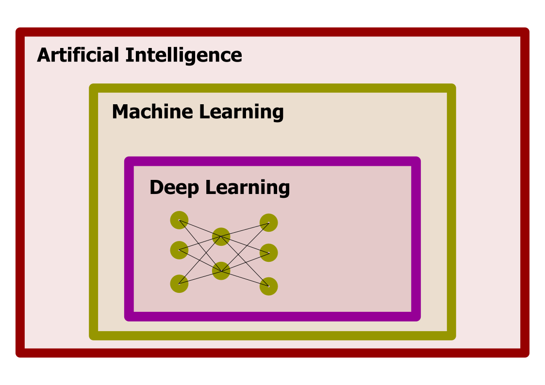
Deep Learning, Machine Learning, and Artificial Intelligence
Deep Learning is part of the area of Machine Learning, a set of techniques to produce models that use examples to build the model, rather than using a hardcoded algorithm. Machine Learning itself is just an area of Artificial Intelligence, an area of computer science dedicated to studying how computers can perform tasks usually considered as intellectual.
Learning from data, a scientific perspective
The idea of learning from data is not foreign to scientist. The objective of science is to create models that explain phenomena and provides predictions that can be confirmed or rejected by experiments or observations.
Scientists create models that not only give us insight about nature but also equations that allow us to make predictions. In most cases, clean equations are simply not possible and we have to use numerical approximations but we try to keep the understanding. Machine Learning is used in cases where mathematical models are known, numerical approximations are not feasible, and we We are satisfied with the answers even if we lost the ability to understand why the parameters of Machine Learning models work the way they do.
In summary, we need 3 conditions for using Machine Learning on a problem:
- Good data
- The existence of patterns on the data
- The lack of a good mathematical model to express the patterns present on the data
Kepler, an example of learning from data
_1971,_MiNr_1649.jpg) |
 |
|---|
 |
|---|
 |
The two shores of Deep Learning
There are two ways to approach Deep Learning. The biological side and the mathematical side.
An Artificial Neural Network (ANN) is a computational model that is loosely inspired by the way biological neural networks in the animal brain process information.
From the other side, they can also be considered as a generalization of the Perceptron idea. A mathematical model for producing functions capable of getting close to a target function via an iterative process.
Both shores serve as good analogies if we are careful not to extrapolate the original ideas beyond their regime of validity. Deep Learning is not pretending to be models of the brain and the complexity of Deep Neural networks is far beyond that of what perceptrons were capable of doing.
Let’s explore these two approaches for a moment.
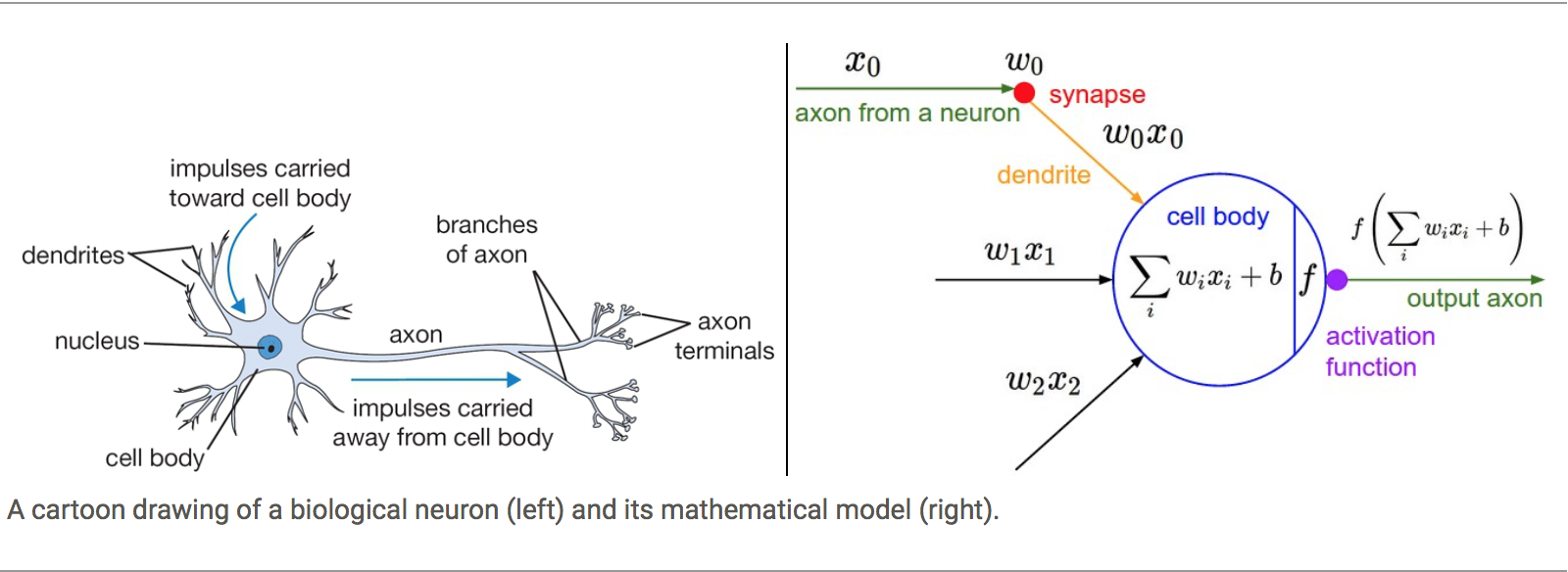
Biological Neural Networks
From one side the idea of simulating synapsis in biological Neural Networks and using the knowledge about activation barriers and multiple connectivities as inspiration to create an Artificial Neural Network. The basic computational unit of the brain is a neuron. Approximately 86 billion neurons can be found in the human nervous system and they are connected with approximately 10¹⁴ — 10¹⁵ synapses

The idea with ANN is that synaptic strengths (the weights w in our mathematical model) are learnable and control the strength of influence and its direction: excitatory (positive weight) or inhibitory (negative weight) of one neuron on another. If the final sum of the different connections is above a certain threshold, the neuron can fire, sending a spike along its axon, which is the output of the network under the provided input.
The Perceptron
The other origin is the idea of Perceptron in Machine Learning.
Perceptron is a linear classifier (binary) and used in supervised learning. It helps to classify the given input data. As a binary classifier, it can decide whether or not an input, represented by a vector of numbers, belongs to some specific class.
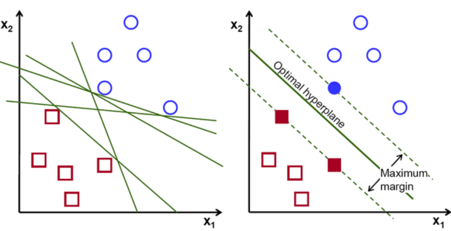
Complexity of Neural Networks
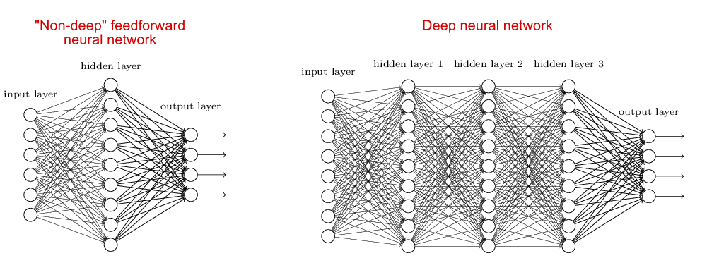
When the neural network has no hidden layer it is just a linear classifier or Perceptron. When hidden layers are added the NN can account for non-linearity, in the case of multiple hidden layers have what is called a Deep Neural Network.
In practice how complex it can be
A Deep Learning model can include:
- Input (With many neurons)
- Layer 1
- …
- …
- Layer N
- Output layer (With many neurons)
For example, the input can be an image with thousands of pixels and 3 colors for each pixel. Hundreds of hidden layers and the output could also be an image. That complexity is responsible for the computational cost of running such networks.
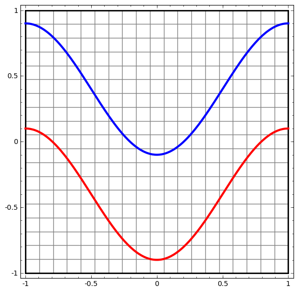
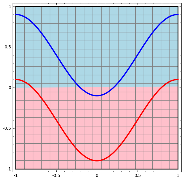
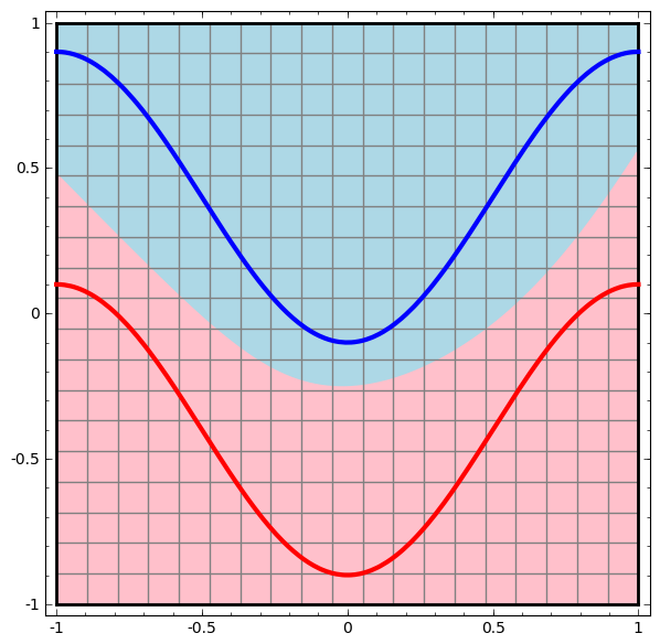
Non-linear transformations with Deep Networks
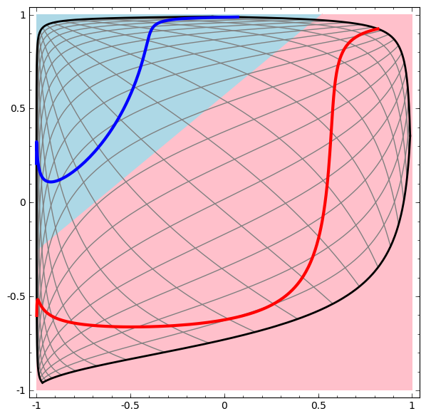
Consider this ilustrative example from this blog: We have two curves, as they are there is no way of creating a straight line that separates both curves. There is however a curve capable of separating the space in two regions where each curve lives on its region. Neural networks approach the problem by transforming the space in a non-linear way, allowing the two curves to be easily separable with a simple line.
 |
 |
 |
|---|---|---|
 |
 |
Dynamic visualization of the transformations
In its basic form, a neural network consists of the application of affine transformations (scalings, skewings and rotations, and translations) followed by pointwise application of a non-linear function:
 |
|---|
 |
 |
|---|
Basic Neural Network Architecture

Neural Network Zoo
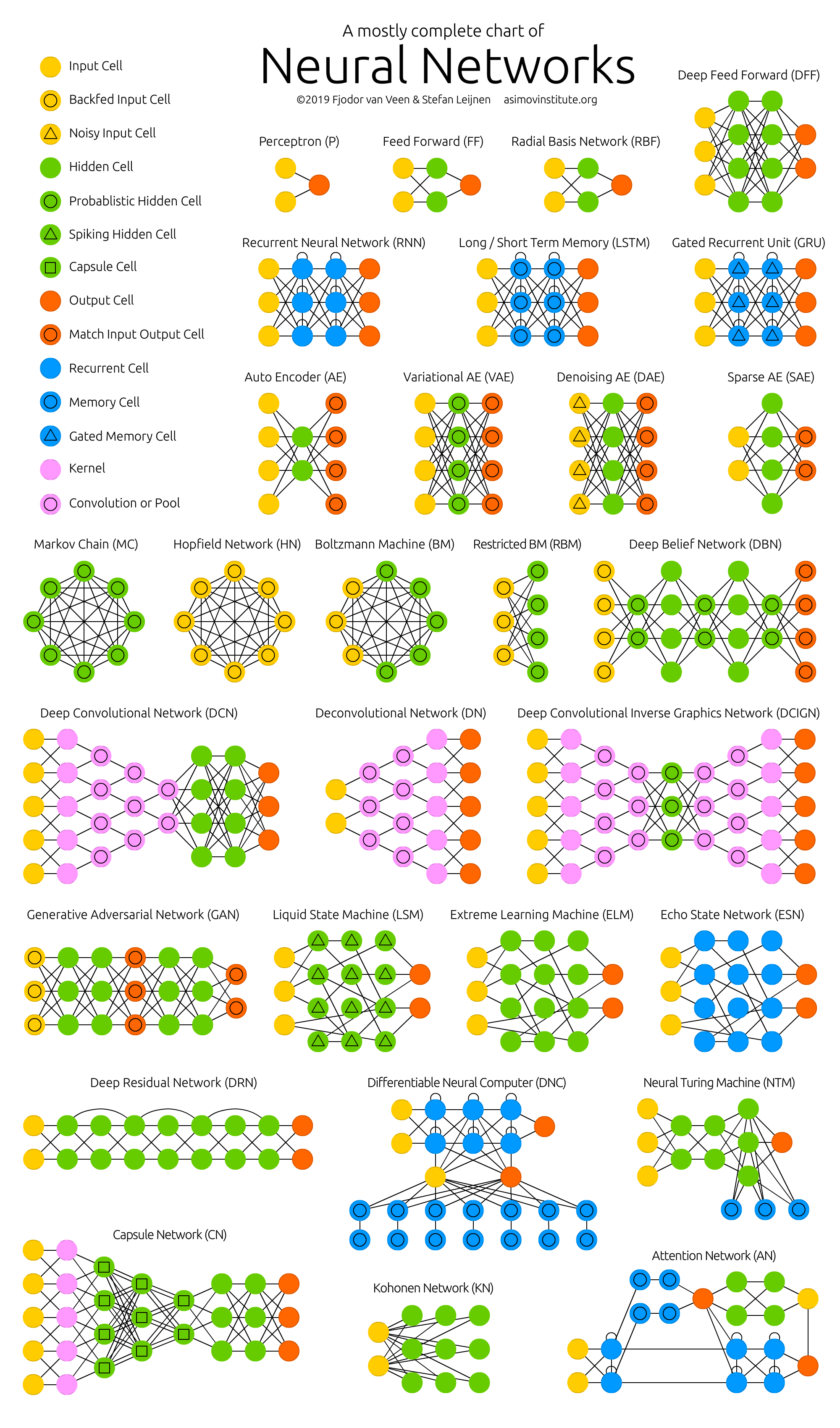
Since neural networks are one of the more active research fields in machine learning, a large number of modifications have been proposed. In the following figure, a summary of the different node structures is drawn and from that, relations and acronyms are provided such that some of the different networks are related someway. The figure below shows a summary but let me give you a quick overview of a few of them.
1) Feed forward neural networks (FF or FFNN) and perceptrons (P). They feed information from the front to the back (input and output, respectively). Neural networks are often described as having layers, where each layer consists of either input, hidden, or output cells in parallel. A layer alone never has connections and in general two adjacent layers are fully connected (every neuron from one layer to every neuron to another layer). One usually trains FFNNs through back-propagation, giving the network paired datasets of “what goes in” and “what we want to have coming out”. Given that the network has enough hidden neurons, it can theoretically always model the relationship between the input and output. Practically their use is a lot more limited but they are popularly combined with other networks to form new networks.
2) Radial basis functions. This network is simpler than the normal FFNN, as the activation function is a radial function. Each RBFN neuron stores a “prototype”, which is just one of the examples from the training set. When we want to classify a new input, each neuron computes the Euclidean distance between the input and its prototype. Roughly speaking, if the input more closely resembles the class A prototypes than the class B prototypes, it is classified as class A.
3) Recurrent Neural Networks (RNN). These networks are designed to take a series of inputs with no predetermined limit on size. They are networks with loops in them, allowing information to persist.
4) Long/short term memory (LSTM) networks. There is a special kind of RNN where each neuron has a memory cell and three gates: input, output, and forget. The idea of each gate is to allow or stop the flow of information through them.
5) Gated recurrent units (GRU) are a slight variation on LSTMs. They have one less gate and are wired slightly differently: instead of an input, output, and forget gate, they have an update gate.
6) Convolutional Neural Networks (ConvNet) is very similar to FFNN, they are made up of neurons that have learnable weights and biases. In a convolutional neural network (CNN, or ConvNet or shift invariant or space invariant) the unit connectivity pattern is inspired by the organization of the visual cortex, Units respond to stimuli in a restricted region of space known as the receptive field. Receptive fields partially overlap, over-covering the entire visual field. The unit response can be approximated mathematically by a convolution operation. They are variations of multilayer perceptrons that use minimal preprocessing. Their wide applications are in image and video recognition, recommender systems, and natural language processing. CNN’s requires large data to train on.
From http://www.asimovinstitute.org/neural-network-zoo
Activation Function
Each internal neuron receives input from several other neurons, computes the aggregate, and propagates the result based on the activation function.

Neurons apply activation functions at these summed inputs.
Activation functions are typically non-linear.
-
The Sigmoid Function produces a value between 0 and 1, so it is intuitive when a probability is desired and was almost standard for many years.
-
The Rectified Linear (ReLU) activation function is zero when the input is negative and is equal to the input when the input is positive. Rectified Linear activation functions are currently the most popular activation function as they are more efficient than the sigmoid or hyperbolic tangent.
-
Sparse activation: In a randomly initialized network, only 50% of hidden units are active.
-
Better gradient propagation: Fewer vanishing gradient problems compared to sigmoidal activation functions that saturate in both directions.
-
Efficient computation: Only comparison, addition, and multiplication.
-
There are Leaky and Noisy variants.
-
-
The Soft Plus shared some of the nice properties of ReLU and still preserves continuity on the derivative.
Inference or Foward Propagation
 |
 |
 |
|---|---|---|
| Receiving Input | Computing Hidden Layer | Computing Output |
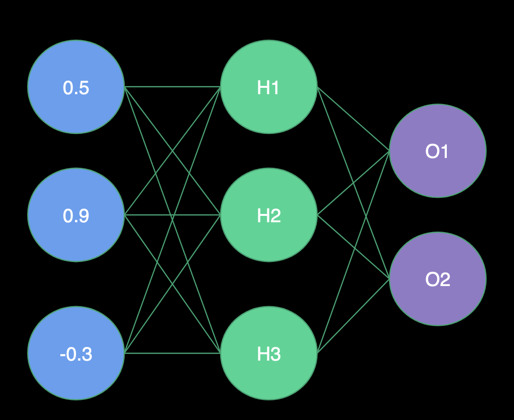
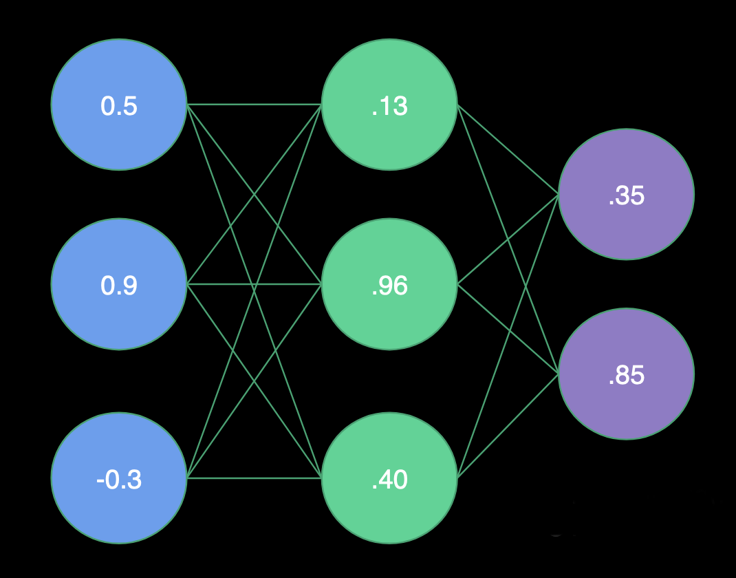
Receiving Input
- H1 Weights = (1.0, -2.0, 2.0)
- H2 Weights = (2.0, 1.0, -4.0)
- H3 Weights = (1.0, -1.0, 0.0)
- O1 Weights = (-3.0, 1.0, -3.0)
- O2 Weights = (0.0, 1.0, 2.0)
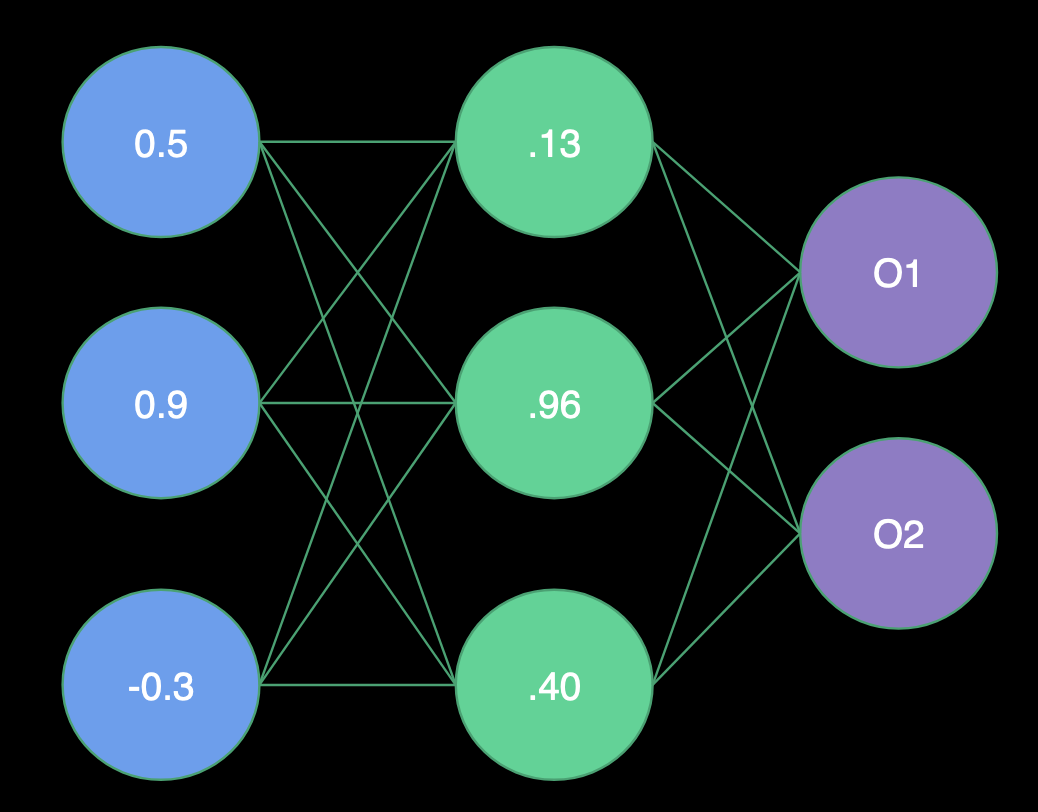
Hidden Layer
- H1 = Sigmoid(0.5 * 1.0 + 0.9 * -2.0 + -0.3 * 2.0) = Sigmoid(-1.9) = .13
- H2 = Sigmoid(0.5 * 2.0 + 0.9 * 1.0 + -0.3 * -4.0) = Sigmoid(3.1) = .96
- H3 = Sigmoid(0.5 * 1.0 + 0.9 * -1.0 + -0.3 * 0.0) = Sigmoid(-0.4) = .40
Output Layer
- O1 = Sigmoid(.13 * -3.0 + .96 * 1.0 + .40 * -3.0) = Sigmoid(-.63) = .35
- O2 = Sigmoid(.13 * 0.0 + .96 * 1.0 + .40 * 2.0) = Sigmoid(1.76) = .85
In terms of Linear Algebra:
[\begin{bmatrix}
1 & -2 & 2
2 & 1 & -4
1 & -1 & 0
\end{bmatrix}
\cdot
\begin{bmatrix}
0.5
0.9
-0.3
\end{bmatrix}
=
\begin{bmatrix}
-1.9
3.1
-0.4
\end{bmatrix}]
The fact that we can describe the problem in terms of Linear Algebra is one of the reasons why Neural Networks are so efficient on GPUs. The same operation as a single execution line looks like this:
Biases
It is also very useful to be able to offset our inputs by some constant. You can think of this as centering the activation function or translating the solution (next slide). We will call this constant the bias, and there will often be one value per layer.
Accounting for Non-Linearity
Neural networks are so effective in classification and regression due to their ability to combine linear and non-linear operations on each step of the evaluation.
- The matrix multiply provides the skew and scale.
- The bias provides the translation.
- The activation function provides the twist.
Training Neural Networks: The backpropagation
During training, once we have forward propagated the network, we will find that the final output differs from the known output. The weights must need to be modified to produce better results in the next attempt.
How do we know which new weights? to use?
We want to minimize the error on our training data. Given labeled inputs, select weights that generate the smallest average error on the outputs. We know that the output is a function of the weights:
[E(w_1,w_2,w_3,…i_1,…t_1,…)]
Just remember that the response of a single neuron can be written as
[f (b + \sum_{i=1}^N a_i w_i),]
where the \(a_i\) is the output of the previous layer (or the input if it is the second layer) and \(w_i\) are the weights. So to figure out which way, we need to change any particular weight, say \(w_3\), we want to calculate
[\frac{\partial E}{\partial {w,i,t}}]
If we use the chain rule repeatedly across layers we can work our way backward from the output error through the weights, adjusting them as we go. Note that this is where the requirement that activation functions must have nicely behaved derivatives comes from.
This technique makes the weight inter-dependencies much more tractable. An elegant perspective on this can be found from Chris Olahat Blog
With basic calculus, you can readily work through the details.
You can find an excellent explanation from the renowned 3Blue1Brown
Solving the back propagation efficiently
The explicit solution for backpropagation leaves us with potentially many millions of simultaneous equations to solve (real nets have a lot of weights).
They are non-linear to boot. Fortunately, this isn’t a new problem created by deep learning, so we have options from the world of numerical methods.
The standard has been Gradient Descent local minimization algorithms.
To improve the convergence of Gradient Descent, refined methods use adaptive time step and incorporate momentum to help get over a local minimum. Momentum and step size are the two hyperparameter
The optimization problem that Gradient Descent solves is a local minimization. We don’t expect to ever find the actual global minimum. Several techniques have been created to avoid a solution being trapped in a local minima.
We could/should find the error for all the training data before updating the weights (an epoch). However, it is usually much more efficient to use a stochastic approach, sampling a random subset of the data, updating the weights, and then repeating with another. This is the mini-batch Gradient Descent
Modern Neural Network Architectures
Convolutional Neural Networks
A convolutional neural network (CNN) is a Deep Learning algorithm that can take in an input image, assign importance (learnable weights and biases) to various aspects/objects in the image, and be able to differentiate one from the other. The pre-processing required in a ConvNet is much lower as compared to other classification algorithms. While in primitive methods filters are hand-engineered, with enough training, ConvNets can learn these filters/characteristics.
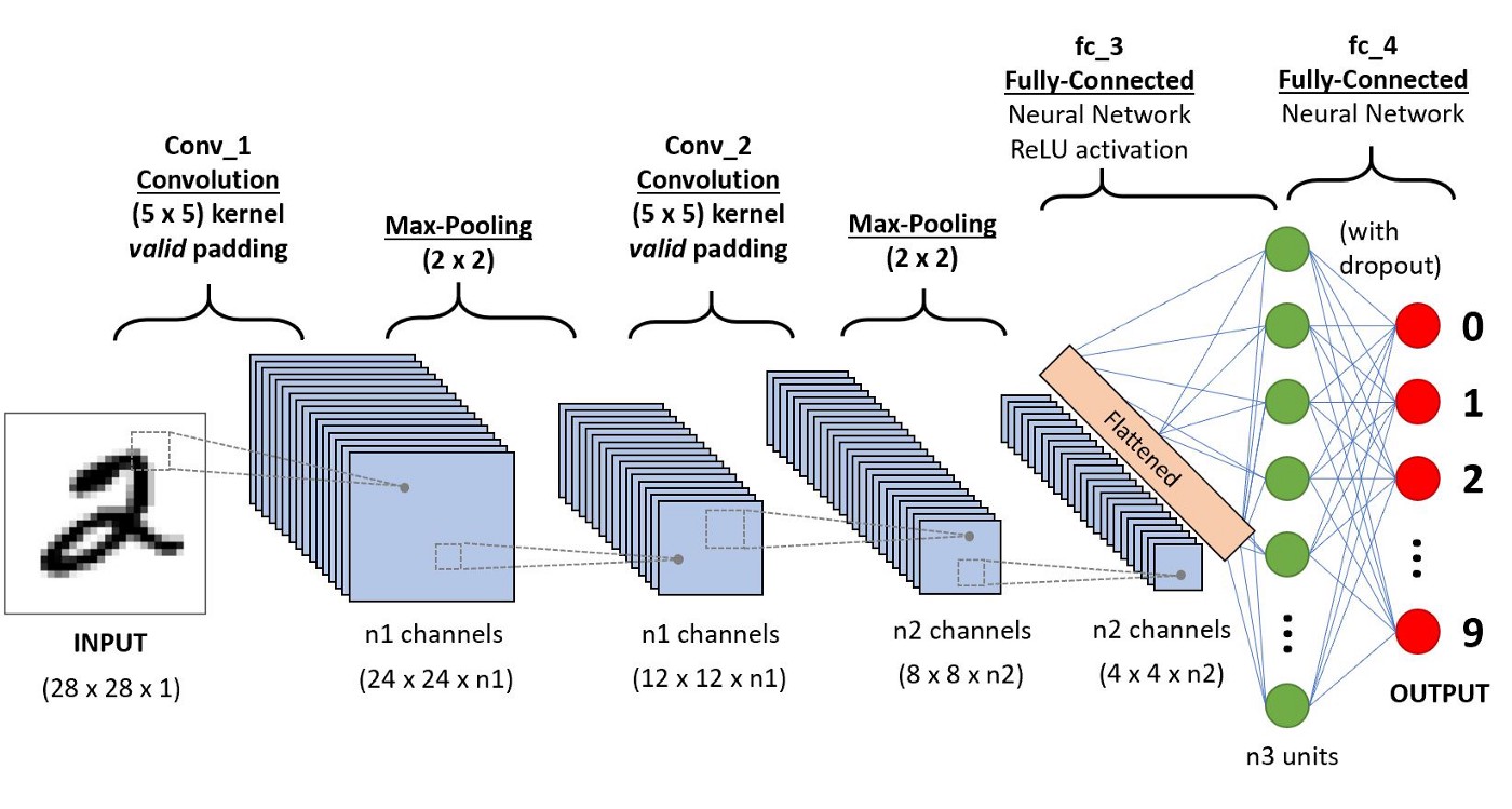
As seen from this figure, CNN consists of several convolutional and subsampling layers optionally followed by fully connected layers.
Let us say that our input to the convolutional layer is a \(m \times m \times r\) pixels in an image where \(m\) is the height and width of the image and \(r\) is the number of channels, e.g. an RGB image has \(r=3\). The convolutional layer will have \(k\) filters (or kernels) of size \(n \times n \times q\) where n is smaller than the dimension of the image and \(q\) can either be the same as the number of channels r or smaller and may vary for each kernel. The size of the filters gives rise to the locally connected structure which is each convolved with the image to produce k feature maps of size \(m−n+1\).
A simple demonstration is shown in the figure below, where we assume a binary picture and a single filter of a 3x3 matrix. The primary purpose of Convolution is to extract features from the input image. Convolution preserves the spatial relationship between pixels by learning image features using small squares of input data. The orange square slide over the figure and for each 3x3 overlap, I multiply every element of the 3x3 submatrix of the figure with the convolution and then I add all elements afterward.
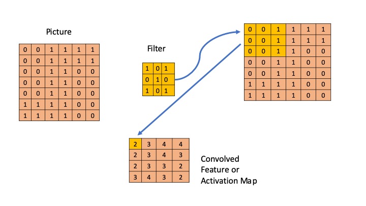
It is clear that different values of the filter matrix will produce different Feature Maps for the same input image.
Typical filter matrices are now described.
For edge detection: \(\begin{bmatrix} 1&0&-1\\ 0&0&0\\ -1&0&1\\ \end{bmatrix} \;\; \begin{bmatrix} 0&1&0\\ 1&-4&1\\ 0&1&0\\ \end{bmatrix} \;\; \begin{bmatrix} -1&-1&-1\\ -1&8&-1\\ -1&-1&-1\\ \end{bmatrix}\)
For sharpen: \(\begin{bmatrix} 0&-1&0\\ -1&5&-1\\ 0&-1&0\\ \end{bmatrix}\)
In practice, a CNN learns the values of these filters on its own during the training process (although we still need to specify parameters such as the number of filters, filter size, architecture of the network, etc. before the training process). The more filters we have, the more image features get extracted, and the better our network becomes at recognizing patterns in unseen images.
The other step that is described in this section is the pooling. Spatial Pooling (also called subsampling or downsampling) reduces the dimensionality of each feature map but retains the most important information. Spatial Pooling can be of different types: Max, Average, Sum, etc.
Graph Neural Network
Before I end and get more into Neural networks and different packages, I would like to discuss one of the most recent proposals in the literature. The so-called Graph Neural Network.
As much of the available information in fields like social networks, knowledge graphs, recommender systems, and even life science comes in the form of graphs, very recently people have developed specific neural networks for these types of applications. Most of the discussion here has been taken from Zhou’s paper.
A Graph Neural Network is a type of Neural Network which directly operates on the Graph structure, which we define by a set of nodes and edges \(G = (V, E)\). A typical application of GNN is node classification. Essentially, every node in the graph is associated with a label, and we want to predict the label of the nodes without ground truth. Here we describe briefly this application and let the reader search for more information.
In the node classification problem setup, each node \(V\) is characterized by its feature \(x_v\) and associated with a ground-truth label \(t_v\). Given a partially labeled graph \(G\), the goal is to leverage these labeled nodes to predict the labels of the unlabeled. It learns to represent each node with a \(d\) dimensional vector (state) \(\vec{h}_V\) which contains the information of its neighborhood. The state embedding \(\vec{h}_V\) is an \(s\)-dimension vector of node \(V\) and can be used to produce an output \(\vec{o}_V\) such as the node label. Let \(f\) be a parametric function, called a local transition function, that is shared among all nodes and updates the node state according to the input neighborhood, and let \(g\) be the local output function that describes how the output is produced. Then, \(\vec{h}_V\) and \(\vec{o}_V\) are defined as follows:
[\vec{h}V = f ( \vec{x}_V, \vec{x}{CO[V]}, \vec{h}{ne[V]}, \vec{x}{ne[V]})]
[\vec{o}_V = g(\vec{h}_V, \vec{x}_V)]
where \(\vec{x}_V\), \(\vec{x}_{co[V]}\), \(\vec{h}_{ne[V]}\), \(\vec{x}_{ne[V]}\) are the features of \(V\), the features of its edges, the states, and the features of the nodes in the neighborhood of \(V\), respectively.
Let \(\vec{H}\), \(\vec{O}\) , \(\vec{X}\) , and \(\vec{X}_N\) be the vectors constructed by stacking all the states, all the outputs, all the features, and all the node features, respectively. Then we have a compact form as: \(\vec{H} = F (\vec{H}, \vec{X})\) \(\vec{O} = G(\vec{H},\vec{X}_N)\) where \(F\), the global transition function, and \(G\), the global output function are stacked versions of f and g for all nodes in a graph, respectively. The value of \(\vec{H}\) is the fixed point of Eq. 3 and is uniquely defined with the assumption that \(F\) is a contraction map. Since we are seeking a unique solution for \(\vec{h}_v\), we can apply Banach fixed point theorem and rewrite the above equation as an iteratively update process. Such operation is often referred to as message passing or neighborhood aggregation. \(\vec{H}^{t+1} = F (\vec{H}^t, \vec{X})\) where \(\vec{H}\) and \(\vec{X}\) denote the concatenation of all the \(\vec{h}\) and \(\vec{x}\), respectively. The output of the GNN is computed by passing the state h_v as well as the feature \(x_v\) to an output function g. \(\vec{o} = g(\vec{h}_V,\vec{x}_V)\)
More details on this methodology can be found in the paper above.
Generative Adversarial Networks
Generative adversarial networks (GANs) are deep neural net architectures comprised of two nets, pitting one against the other (thus the “adversarial”). Introduced in 2014 by Goodfellow and other people.
GANs’ potential is huge because they can learn to mimic any distribution of data. That is, GANs can be taught to create worlds eerily similar to our own in any domain: images, music, speech, prose.
To understand GANs, you should know how generative algorithms work. Up to now, most of the algorithms we have discussed are the so-called discriminative algorithms, where we try to predict the output from a given set of features.
In the Bayesian language, we are trying to predict
\(P(c_j ; x_1,x_2,\cdots,x_n)\).
In GANs, we are concerned with a different idea,
We try two features given a certain label.
Therefore, here we would like to build
\(P(x_1,x_2,\cdots,x_n ; c_j)\).
The idea in GANs then is to have two neural networks. One is called the generator, which generates features, and the other network, the discriminator evaluates its authenticity, i.e. the discriminator decides whether each instance of data that it reviews belongs to the actual training dataset or not. For example, we try to analyze a book by a great author (for example Garcia Marquez). We could analyze the language used in his texts but for this example, the generator should be able to create words and the discriminator should be able to recognize if these are authentic. The idea of the generator then is to create words that were not created by Garcia Marquez but that the discriminator is unable to distinguish.
Milestones of Neural Networks and Deep Learning Frameworks
The history
Artificial Intelligence is born
The term Artificial Intelligence (AI) was first coined by John McCarthy in 1956. In the early days, the focus was on hard coding rules that computers can follow via inference. That was called the age on symbolic AI and let to the expert systems of the 80s and early 90s.
Deep Learning old names
Deep Learning has received different names over time. It was called Cybernetics in the 70s, Connectionism in the 80s. Neural Networks in the 90s and today we call it Deep Learning
First DL Frameworks from 2000’s to 2012
- First high-level tools such as MATLAB, OpenNN, and Torch.
- They were not tailored specifically for neural network model development or having complex user APIs
- No GPU support.
- Machine Learning practitioners do a lot of manual manipulations for the input and output.
- Limited capability for complex networks.
AlexNet in 2012
-
In 2012, Alex Krizhevsky et al. from the University of Toronto proposed a deep neural network architecture later known as AlexNet that achieved impressive accuracy on ImageNet dataset and outperformed the second-place contestant by a large margin. This outstanding result sparked excitement in deep neural networks after a long time of being considered the
- Alex Krizhevsky et al., ImageNet Classification with Deep Convolutional Neural Networks (2012), NeurIPS 2012
- Deep Learning frameworks were born such as Caffe, Chainer and Theano.
- Users could conveniently build more complex deep neural network models such as CNN, RNN, and LSTM.
- Single GPU first and soon after multi-GPU training was supported which significantly reduced the time to train these models and enabled training large models that were not able to fit into a single GPU memory earlier.
- Caffe and Theano used a declarative programming style while Chainer adopted the imperative programming style.
Big Tech companies jump in
- After the success of AlexNet drew great attention in the area of computer vision and reignited the hope of neural networks, large tech companies joined the force of developing deep learning frameworks.
- Google open sourced the famous TensorFlow framework that is still the most popular deep learning framework in the ML field up to date.
- Facebook hired the inventor of Caffe and continued the release of Caffe2; at the same time, Facebook AI Research (FAIR) team also released another popular framework PyTorch which was based on the Torch framework but with the more popular Python APIs.
- Microsoft Research developed the CNTK framework.
-
Amazon adopted MXNet from Apache, a joint academic project from the University of Washington, CMU, and others.
- TensorFlow and CNTK borrowed the declarative programming style from Theano whereas PyTorch inherited the intuitive and user-friendly imperative programming style from Torch.
- While imperative programming style is more flexible (such as defining a while loop etc.) and easy to trace, declarative programming style often provides more room for memory and runtime optimization based on computing graph.
- MXNet, dubbed as “mix”-net, enjoyed the benefits of both worlds by supporting both a set of symbolic (declarative) APIs and a set of imperative APIs at the same time and optimized the performance of models described using imperative APIs via a method called hybridization.
ResNet in 2016
- In 2015 ResNet was proposed by Kaiming He et al. and again pushed the boundary of image classification by setting another record in ImageNet accuracy.
- Kaiming He et al., Deep Residual Learning for Image Recognition (2016), CVPR 2016
- Industry and academia realized that deep learning was going to be the next big technology trend to solve challenges in various fields that were not deemed possible before.
- Deep Learning frameworks were polished to provide clear-defined user APIs, optimized for multi-GPU training and distributed training and spawned many model zoos and toolkits that were targeted to specific tasks such as computer vision, natural language processing, etc.
- François Chollet almost single-handedly developed the Keras framework that provides a more intuitive high-level abstraction of neural networks and building blocks on top of existing frameworks such as TensorFlow and MXNet.
- Keras became the de facto model level APIs in TensorFlow 2.x.
Consolidating Deep Learning Frameworks
- Around 2019 start a period of consolidation in the area of Deep Learning frameworks with the duopoly of two big “empires”: TensorFlow and PyTorch.
- PyTorch and TensorFlow represent more than 90% of the use cases of deep learning frameworks in research and production.
- Theano, primarily developed by the Montreal Institute for Learning Algorithms (MILA) at the Université de Montréal is no longer actively developed and the last version is from 2020.
- Chainer team transitioned their development effort to PyTorch in 2019.
- Microsoft stopped active development of the CNTK framework and part of the team moved to support PyTorch on Windows and ONNX runtime.
- Keras was assimilated by TensorFlow and became one of its high-level APIs in the TensorFlow 2.0 release.
- MXNet remained a distant third in the deep learning framework space.
Doing Deep Learning at large
- Large model training is a new trend in 2020 to our days.
- With the birth of BERT [3] and its Transformer-based relatives such as GPT-3 [4], the ability to train large models became a desired feature of deep learning frameworks.
- Jacob Devlin et al., BERT: Pre-training of Deep Bidirectional Transformers for Language Understanding (2018)
- Tom B. Brown et al., Language Models are Few-Shot Learners (2020), NeurIPS 2020
- Now training takes place at a scale up to hundreds if not thousands of GPU devices and custom accelerators.
- Deep learning frameworks adopted the imperative programming style for their flexible semantics and easy debugging.
- To compensate for performance frameworks also provide user-level decorators or APIs to achieve high performance through some JIT (just-in-time) compiler techniques.
Current trends
- Compiler-based operator optimization: Operator kernels are usually implemented manually or via some third-party libraries such as BLAS, CuDNN, or OneDNN. There are challenges associated with the movement from development to production. In addition, the growth of new deep learning algorithms is often much faster than the iteration of these libraries making new operators often not supported by these libraries.
- Deep learning compilers: Apache TVM, MLIR, Facebook Glow, etc. have been proposed to optimize and run computations efficiently on any hardware backend. They are well positioned to serve as the entire backend stack in the deep learning frameworks.
- Unified API standards: Since the majority of machine learning practitioners and data scientists are familiar with the NumPy library, this is the de-facto standard for multidimensional array manipulation. Still, at other levels, many deep learning frameworks share similar but slightly different user APIs. JAX is NumPy on the CPU, GPU, and TPU, with great automatic differentiation for high-performance machine learning research. It likely became a superset of NumPy with agnostic operation on many devices.
- Transparent Multi-node or multi-device training: New frameworks such as OneFlow, treat data communication as part of the overall computation graph of the model training. Data movement optimization is central for multiple training strategies (single device vs multi-device vs distributed training) as the previous deep learning frameworks do, it can provide a simpler user interface with better performance.
Key Points
Deep Learning are techniques to explore multiple level of data transformations
Deep Learning is usually understood as the use of neural network models
Neural network models can be trained efficiently using GPUs
Three popular Deep Learning models are TensorFlow, PyTorch and MXNet
Molecular Dynamics
Overview
Teaching: 60 min
Exercises: 0 minQuestions
What is Classical Molecular Dynamics (CMD)?
How can we simulate the motion of particles subject to inter-particle forces?
Which problems can be solved with CMD?
How we can use GPUs to accelerate a CMD simulation
Objectives
Learn the basics of Molecular Dynamics
Learn how to use several CMD packages that can use GPUs to accelerate simulations
We can solve Newton’s equations of motion for relative motion of atoms subject to intramolecular forces.
Molecular Dynamics simulations provide a powerful tool for studying the motion of atomic, molecular, and nanoscale systems (including biomolecular systems). In molecular dynamics simulation, the motion of the atoms is treated with classical mechanics; this means that the positions and velocities/momenta of the atoms are well-defined quantities. This in contrast with quantum mechanics where the theory sets limits to the ability to measure both quantities precisely.
In classical molecular dynamics, positions and velocities are quantities updated using Newton’s laws of motion (or equivalent formulations).
The motion of the atoms over the duration of a molecular dynamics simulation is known as a trajectory. The analysis of molecular dynamics trajectories can provide information about thermodynamic and kinetic quantities relevant to your system, and can also yield valuable insights into the mechanism of processes that occur over time. Thus molecular dynamics simulations are employed to study an enormous range of chemical, material, and biological systems.
One of the central quantities in a molecular dynamics simulation comes from the inter-particle forces. From Newton’s second law, we know that the acceleration a particle feels is related to the force it experiences;
[\vec{F} = m \vec{a}.]
The acceleration of each particle in turn determines how the position and momentum of each particle change. Therefore, the trajectories one observes in a molecular dynamics simulation are governed by the forces experienced by the particles being simulated.
We will derive this force from the potential curve as follows,
[F(r) = -\frac{d}{dr} V(r),]
where \(V(r)\) denotes the potential as a function of the bond length that can be readily computed.
The potential function can be computed directly from quantum mechanical calculations, which we call those ab initio calculations. The alternative is to use approximations of the values we will get otherwise will be computed from running quantum mechanical equations. We call these approximations “force fields” and the resulting equations are called force-field molecular dynamics or Classical Molecular Dynamics (CMD).
There is a variety of computer algorithms available that permit Newton’s Law to be solved for many thousands of atoms even with modest computational resources. A classical algorithm for propagating particles under Newton’s laws is called the Velocity Verlet algorithm.
This algorithm updates the positions and velocities of the particles once the forces have been computed. Using the Velocity Verlet algorithm, the position of the \(i^{th}\) particle is updated from time \(t\) to time \(t+dt\) according to equation:
[\vec{r}_i (t+dt) = \vec{r}_i (t) + \vec{v}_i(t) dt + \frac{1}{2} \vec{a}_i (t) dt^2]
where \(\vec{r}_i(t)\) represents the position vector of the \(i^{th}\) particle at time \(t\), \(\vec{v}_i(t)\) represents the velocity vector of the \(i^{th}\) particle at time \(t\), and, \(\vec{a}_i(t)\) represents the acceleration vector of the \(i^{th}\) particle at time \(t\). A MD code could use a Cartesian coordinate system so \(r\) has an \(x\), \(y\), and \(z\) component: \(\vec{r} = r_x \hat{x} + r_y \hat{y} + r_z \hat{z}\) and similarly for \(\vec{r}\) and \(\vec{a}\). In the previous expression, \(\hat{x}\) is the unit vector along the \(x\)-axis. The velocity of the \(t^{th}\) particle is updated from time \(t\) to time \(t+dt\) according to
[\vec{v}_i (t+dt) = \vec{v}_i(t) + \frac{1}{2}\left( \vec{a}_i (t) + \vec{a}_i (t+dt) \right) dt]
and the acceleration comes from Newton’s \(2^{nd}\) law, \(\vec{a}_i = \frac{\vec{F_i}}{m_i}\). Note that in the equation above, \(\vec{a}_i (t)\) indicates the accelerations before the particle positions are updated and \(\vec{a}_i (t+dt)\) indicates the accelerations after the particle positions are updated.
Hence, the velocity Verlet algorithm requires two force calculations and two calculations of the accelerations for each iteration in the simulation.
Practical application of the Velocity Verlet algorithm requires the specification of an initial position and initial velocity for each particle. In this work, the initial positions are specified by arranging the atoms in a simple cubic lattice, and the initial velocities are assigned based on the Maxwell-Boltzmann distribution corresponding to a user-supplied initial temperature.
A key ingredient in a molecular dynamics simulation is the potential energy function, also called the force field. This is the mathematical model that describes the potential energy of the simulated system as a function of the coordinates of its atoms. The potential energy function should be capable of faithfully describing the attractive and repulsive interparticle interactions relevant to the system of interest. For simulations of complex molecular or biomolecular systems with many different atom types, the potential energy function may be quite complicated, and its determination may itself be a subject of intense research.
Because we are interested in simulating monatomic gasses, we use a particularly simple potential energy function in our simulation known as the Lennard-Jones potential, which was also used in Rahman’s original work,
[U(r_{ij}) = 4 \epsilon \left( \left(\frac{\sigma}{r_{ij}}\right)^{12} - \left(\frac{\sigma}{r_{ij}}\right)^{6} \right)]
The Lennard-Jones potential is defined by two parameters, \(\epsilon\), and \(\sigma\), which may be determined by fitting simulations to experimental data, through ab initio calculations, or by a combination of experiment and calculation. The parameter \(\epsilon\) is related to the strength of the interparticle interactions and has dimensions of energy. The value of \(\epsilon\) manifests itself as the minimum value of the potential energy between a pair of particles, \(min(U(r_{ij}))= -\epsilon\).
The parameter \(\sigma\) is related to the effective size of the particles and has dimensions of length. In effect, the value of \(\sigma\) determines at which separations attractive forces dominate and at which separations repulsions dominate.
For example, the value of \(\sigma\) determines the interparticle separation that minimizes the Lennard- Jones potential by the relation \(r_{min} = 2^{\frac{1}{6}}\sigma\) where \(U(r_{min}) = \epsilon\).
In the case of Lennard-Jone’s potential, only the scalar separation between a pair of particles is needed to determine the potential energy of the pair within the Lennard-Jones model.
The total potential energy of the system of \(N\) particles is simply the sum of the potential energy of all unique pairs. This potential neglects orientation effects which may be important for describing molecules that lack spherical symmetry and also neglects polarization effects which may arise in many chemically relevant situations, water for example. Lennard-Jones parameters for various noble gasses are provided in the table below.
| Particle | m (kg) | \(\sigma (m)\) | \(\epsilon (J)\) |
|---|---|---|---|
| Helium | \(6.646 \times 10^{27}\) | \(2.64 \times 10^{10}\) | \(1.50 \times 10^{22}\) |
| Neon | \(3.350 \times 10^{26}\) | \(2.74 \times 10^{10}\) | \(5.60 \times 10^{22}\) |
| Argon | \(6.633 \times 10^{26}\) | \(3.36 \times 10^{10}\) | \(1.96 \times 10^{21}\) |
| Krypton | \(1.391 \times 10^{26}\) | \(3.58 \times 10^{10}\) | \(2.75 \times 10^{21}\) |
| Xeon | \(2.180 \times 10^{26}\) | \(3.80 \times 10^{10}\) | \(3.87 \times 10^{21}\) |
Once the potential energy function has been specified, the forces on the particles may be calculated from the derivative on the potential energy function with respect to interparticle separation vectors:
[\vec{𝐹}i = − \sum{j\neq i}^{N} \frac{\partial U(\vec{r}{ij})}{\partial \vec{r}{ij}}]
That is, each particle experiences a unique force from each of the remaining particles in the system. Each unique force is related to the derivative of the potential energy with respect to the separation vector of the particle pair,
[\vec{F}{ij}(\vec{r}{ij}) = \frac{24\epsilon}{\sigma^2} \vec{r}{ij} \left( 2\left( \frac{\sigma}{\vec{r}{ij}} \right)^{14} - \left( \frac{\sigma}{\vec{r}_{ij}} \right)^{8} \right)]
Note that, unlike the potential energy, the pair force is fundamentally a vector quantity and has a direction associated with it. We note that the two \(\frac{\sigma}{\vec{r}_{ij}}\) terms in the force can be equivalently evaluated in terms of the scalar separation, \(\vec{r}_{ij}\), because they contain even powers of the separation vector, and even powers of the separation vector are equivalent to the same even power of the scalar separation.
Because the Lennard-Jones potential has a minimum at the separation \(r_{min} = 2^{\frac{1}{6}}\sigma\), the force goes to zero at separation \(r_{min}\).
Once all the unique pair force vectors \(\vec{F}_{ij}\) are determined from evaluation of based on the coordinates of the system, the total force vector \(\vec{F}_i\) acting on the \(i^{th}\) particle is computed as the sum over all the unique pair forces. Hence, the potential energy function is a key ingredient in determining the dynamics through its impact on the forces, and therefore, the instantaneous position and velocity.
The instantaneous positions and velocities of the particles constitute the raw data generated by a molecular dynamics simulation. These trajectories may be directly visualized, and a variety of physical quantities can be derived from information contained in these trajectories.
LAMMPS
LAMMPS is a C++ code for classical molecular dynamics with a focus on material modeling. It is an acronym for Large-scale Atomic/Molecular Massively Parallel Simulator It is also a free software optimized for OPENMP, OPENMPI and CUDA libraries. The code is flexible in order to simulate various physical situations and can perform simulation with many different algorithms. The price to pay is to write an input script file which defines all parameters as well as the quantities to be monitored.
There are many parameters that can be set on LAMMPS All possibilities can be found in the software manual at LAMMPS MANUAL. The last version of the manual (Release 15Jun2023) contains 2786 pages, which illustrates the complexity of the software. To start with LAMMPS is not always easy, and if you are a beginner you must follow the basic instructions and understand the meaning of the lines of a script file. The goal of this session is to illustrate the versatility of the software and the quality of the parallelization.
The binary file is called lmp.
In order to have a brief description of LAMMPS. type lmp -help.
You will learn how the software has been compiled and all methods are available.
If some options are missing, you can download the source tarball and compile the software with the options you can
use with your computer. See the appendix for an installation.
You can start a simulation by using the command
$> lmp -in in.system
where in.system is a script file defining the system (particle types, ensemble, forces,
boundary conditions,…), the different observables to be calculated, and different correlation
functions (static and dynamic).
Lennard-Jones Liquid
We will use this first example of a LAMMPS input file
  # 3d Lennard-Jones melt

  variable	x index 1
  variable	y index 1
  variable	z index 1

  variable	xx equal 50*$x
  variable	yy equal 50*$y
  variable	zz equal 50*$z

  units		lj
  atom_style	atomic

  lattice		fcc 0.8442
  region		box block 0 ${xx} 0 ${yy} 0 ${zz}
  create_box	1 box
  create_atoms	1 box
  mass		1 1.0

  velocity	all create 1.44 87287 loop geom

  pair_style	lj/cut 2.5
  pair_coeff	1 1 1.0 1.0 2.5

  neighbor	0.3 bin
  neigh_modify	delay 0 every 20 check no

  fix		1 all nve

  run		300
This input will simulation an Atomic fluid of particles following Lennard-Jones potential. In its original version the parameters are:
- 32,000 atoms for 100 timesteps
- reduced density = 0.8442 (liquid)
- force cutoff = 2.5 sigma
- neighbor skin = 0.3 sigma
- neighbors/atom = 55 (within force cutoff)
- NVE time integration
We can explore the variables used here
units
This command sets the style of units used for a simulation. It determines the units of all quantities specified in the input script and data file, as well as quantities output to the screen, log file, and dump files. Typically, this command is used at the very beginning of an input script.
We are running a unitless simulation for a Lennard-Jones potential. For style lj, all quantities are unitless. Without loss of generality, LAMMPS sets the fundamental quantities mass, \(\sigma\) , \(\epsilon\), and the Boltzmann constant \(k_B = 1\). The masses, distances, energies you specify are multiples of these fundamental values.
atom_style
Define what style of atoms to use in a simulation. This determines what attributes are associated with the atoms. This command must be used before a simulation is setup via a read_data, read_restart, or create_box command.
We are using atom_style atomic because we are dealing with point-like particles.
The choice of style affects what quantities are stored by each atom, what quantities are
communicated between processors to enable forces to be computed, and what quantities are
listed in the data file read by the read_data command.
lattice
A lattice is a set of points in space, determined by a unit cell with basis atoms, that is replicated infinitely in all dimensions.
A lattice is used by LAMMPS in two ways. First, the create_atoms command creates atoms on the
lattice points inside the simulation box. Note that the create_atoms command allows different
atom types to be assigned to different basis atoms of the lattice.
In our case, we have particles under a reduced density of 0.8442.
region
This command defines a geometric region of space. Various other commands use regions. For example, the region can be filled with atoms via the create_atoms command. Or a bounding box around the region, can be used to define the simulation box via the create_box command.
The region is identified with the name “box” and for style block, the indices from 1 to 6 correspond to the xlo, xhi, ylo, yhi, zlo, zhi surfaces of the block.
create_box
This command creates a simulation box based on the specified region. Thus a region command must first be used to define a geometric domain. It also partitions the simulation box into a regular 3d grid of rectangular bricks, one per processor, based on the number of processors being used and the settings of the processors command.
We will have just one box in the region that we defined.
create_atoms
This command creates atoms (or molecules) within the simulation box, either on a lattice, or a single atom (or molecule), or on a surface defined by a triangulated mesh, or a random collection of atoms (or molecules).
For the box style, the create_atoms command fills the entire simulation box with particles on the lattice.
mass
Set the mass for all atoms of one or more atom types. Per-type mass values can also be set in the read_data data file using the “Masses” keyword. See the units command for what mass units to use.
We only have one type of atoms and the mass is unitless for lj
velocity
Set or change the velocities of a group of atoms in one of several styles. For each style, there are required arguments and optional keyword/value parameters.
In our case we are associating random values of velocity for all the particles. The create style generates an ensemble of velocities using a random number generator with the specified seed at the specified temperature.
pair_style
Set the formula LAMMPS uses to compute pairwise interactions. The particles in our simulation box are all suject to pair-wise interactions with an energy cutoff of \(2.5 \sigma\)
pair_coeff
Specify the pairwise force field coefficients for one or more pairs of atom types.
fix 1 nve
Perform plain time integration to update position and velocity for atoms in the group each timestep. This creates a system trajectory consistent with the microcanonical ensemble (NVE) provided there are (full) periodic boundary conditions and no other “manipulations” of the system (e.g. fixes that modify forces or velocities).
The primary macroscopic variables of the microcanonical ensemble are the total number of particles in the system N, the system’s volume V, as well as the total energy in the system E. Each of these is assumed to be constant in the ensemble.
run
This command tell us to compute the trajectory during a given number of iterations. In this case we set 300 steps
How to run LAMMPS using GPUs
Submit a request for an interactive job:
$> srun -p comm_gpu_inter -G 3 -t 2:00:00 -c 24 --pty bash
With this command, the partition will be -p comm_gpu_inter. We are requesting 3 GPUs (-G 3)
during 2 hours -t 2:00:00 with 24 CPU cores -c 24 and bash on the shell --pty bash.
Once you get access to the compute node, load singularity.
$> module load singularity
Check the GPUs that you received:
$ nvidia-smi
Tue Aug  1 07:51:25 2023
+---------------------------------------------------------------------------------------+
| NVIDIA-SMI 530.30.02              Driver Version: 530.30.02    CUDA Version: 12.1     |
|-----------------------------------------+----------------------+----------------------+
| GPU  Name                  Persistence-M| Bus-Id        Disp.A | Volatile Uncorr. ECC |
| Fan  Temp  Perf            Pwr:Usage/Cap|         Memory-Usage | GPU-Util  Compute M. |
|                                         |                      |               MIG M. |
|=========================================+======================+======================|
|   0  Quadro RTX 6000                 Off| 00000000:12:00.0 Off |                    0 |
| N/A   29C    P8               22W / 250W|      0MiB / 23040MiB |      0%   E. Process |
|                                         |                      |                  N/A |
+-----------------------------------------+----------------------+----------------------+
|   1  Quadro RTX 6000                 Off| 00000000:13:00.0 Off |                    0 |
| N/A   28C    P8               24W / 250W|      0MiB / 23040MiB |      0%   E. Process |
|                                         |                      |                  N/A |
+-----------------------------------------+----------------------+----------------------+
|   2  Quadro RTX 6000                 Off| 00000000:48:00.0 Off |                    0 |
| N/A   27C    P8               12W / 250W|      0MiB / 23040MiB |      0%   E. Process |
|                                         |                      |                  N/A |
+-----------------------------------------+----------------------+----------------------+

+---------------------------------------------------------------------------------------+
| Processes:                                                                            |
|  GPU   GI   CI        PID   Type   Process name                            GPU Memory |
|        ID   ID                                                             Usage      |
|=======================================================================================|
|  No running processes found                                                           |
+---------------------------------------------------------------------------------------+
One important piece of information about GPUs is the Compute Capability.
The compute capability of a device is represented by a version number, also sometimes called its “SM version”. This version number identifies the features supported by the GPU hardware and is used by applications at runtime to determine which hardware features and/or instructions are available on the present GPU.
All the GPUs are Quadro RTX 6000. These GPUs have Compute Capability 7.5. See more about compute capabilities on the CUDA documentation and the tables with the SM of various GPU cards on this table.
Open a shell on the container:
$> singularity shell --nv /shared/containers/NGC_LAMMPS_patch_3Nov2022.sif
Singularity>
The image NGC_LAMMPS_patch_3Nov2022.sif has been optimized by NVIDIA for running LAMMPS on GPUs.
There are several binaries inside depending on the Compute Capabilities of the GPU.
We need to adjust the environment variables $PATH and $LD_LIBRARY_PATH according to the
SM number of the card.
As the SM number for QUADRO RTX 6000 is 7.5 we can set those variables like this:
Singularity> export PATH=/usr/local/lammps/sm75/bin:$PATH
Singularity> export LD_LIBRARY_PATH=/usr/local/lammps/sm75/lib:$LD_LIBRARY_PATH
With this we are ready to launch LAMMPS. The binary is called lmp. See for example the help
message from the command, execute:
Singularity> mpirun lmp -help

Large-scale Atomic/Molecular Massively Parallel Simulator - 3 Nov 2022

Usage example: lmp -var t 300 -echo screen -in in.alloy

List of command line options supported by this LAMMPS executable:

-echo none/screen/log/both  : echoing of input script (-e)
-help                       : print this help message (-h)
-in none/filename           : read input from file or stdin (default) (-i)
-kokkos on/off ...          : turn KOKKOS mode on or off (-k)
-log none/filename          : where to send log output (-l)
-mdi '<mdi flags>'          : pass flags to the MolSSI Driver Interface
-mpicolor color             : which exe in a multi-exe mpirun cmd (-m)
-cite                       : select citation reminder style (-c)
-nocite                     : disable citation reminder (-nc)
-nonbuf                     : disable screen/logfile buffering (-nb)
-package style ...          : invoke package command (-pk)
-partition size1 size2 ...  : assign partition sizes (-p)
-plog basename              : basename for partition logs (-pl)
-pscreen basename           : basename for partition screens (-ps)
-restart2data rfile dfile ... : convert restart to data file (-r2data)
-restart2dump rfile dgroup dstyle dfile ...
                            : convert restart to dump file (-r2dump)
-reorder topology-specs     : processor reordering (-r)
-screen none/filename       : where to send screen output (-sc)
-skiprun                    : skip loops in run and minimize (-sr)
-suffix gpu/intel/opt/omp   : style suffix to apply (-sf)
-var varname value          : set index style variable (-v)

OS: Linux "Ubuntu 20.04.5 LTS" 3.10.0-1160.24.1.el7.x86_64 x86_64

Compiler: GNU C++ 10.3.0 with OpenMP 4.5
C++ standard: C++14
MPI v3.1: Open MPI v4.1.3rc2, package: Open MPI root@95f4f5de9494 Distribution, ident: 4.1.3rc2, repo rev: v4.1.3, Unreleased developer copy

Accelerator configuration:

KOKKOS package API: CUDA Serial
KOKKOS package precision: double
OPENMP package API: OpenMP
OPENMP package precision: double
There are two variables we will use for executing LAMMPS.
Singularity> gpu_count=3
Singularity> input=in.lj.txt
Execute LAMMPS:
Singularity> mpirun -n ${gpu_count} lmp -k on g ${gpu_count} -sf kk -pk kokkos cuda/aware on neigh full comm device binsize 2.8 -var x 8 -var y 4 -var z 8 -in ${input}
On this command line we are running LAMMPS using MPI launching 3 MPI processes.
The number of processes matches the number of GPUs mpirun -n ${gpu_count}
To use GPUs LAMMPS relies on Kokkos. Kokkos is a templated C++ library that provides abstractions to allow a single implementation of an application kernel (e.g. a pair style) to run efficiently on different kinds of hardware, such as GPUs, Intel Xeon Phis, or many-core CPUs. See more on Kokkos documentation page
Use the “-k” command-line switch to specify the number of GPUs per node. Typically the -np setting of the mpirun command should set the number of MPI tasks/node to be equal to the number of physical GPUs on the node.
In our case we have -k on g ${gpu_count}
The suffix to the style is kk for the particles to be accelerated with GPUs Our simulation is creating more than 27 million atoms:
LAMMPS (3 Nov 2022)
KOKKOS mode is enabled (src/KOKKOS/kokkos.cpp:106)
  will use up to 3 GPU(s) per node
  using 1 OpenMP thread(s) per MPI task
Lattice spacing in x,y,z = 1.6795962 1.6795962 1.6795962
Created orthogonal box = (0 0 0) to (403.10309 201.55154 403.10309)
  1 by 1 by 3 MPI processor grid
Created 27648000 atoms
  using lattice units in orthogonal box = (0 0 0) to (403.10309 201.55154 403.10309)
  create_atoms CPU = 3.062 seconds
At the end of the simulation you get some stats about the performance
Performance: 4270.015 tau/day, 9.884 timesteps/s, 273.281 Matom-step/s
73.6% CPU use with 3 MPI tasks x 1 OpenMP threads

MPI task timing breakdown:
Section |  min time  |  avg time  |  max time  |%varavg| %total
---------------------------------------------------------------
Pair    | 0.20305    | 0.20387    | 0.20487    |   0.2 |  0.67
Neigh   | 4.7754     | 4.8134     | 4.837      |   1.2 | 15.86
Comm    | 2.1789     | 2.2052     | 2.2234     |   1.3 |  7.27
Output  | 0.00077292 | 0.021803   | 0.037289   |  10.4 |  0.07
Modify  | 22.898     | 22.92      | 22.941     |   0.4 | 75.52
Other   |            | 0.1868     |            |       |  0.62

Nlocal:      9.216e+06 ave 9.21655e+06 max 9.21558e+06 min
Histogram: 1 0 0 1 0 0 0 0 0 1
Nghost:         811154 ave      811431 max      810677 min
Histogram: 1 0 0 0 0 0 0 0 1 1
Neighs:              0 ave           0 max           0 min
Histogram: 3 0 0 0 0 0 0 0 0 0
FullNghs:  6.90671e+08 ave 6.90734e+08 max 6.90632e+08 min
Histogram: 1 1 0 0 0 0 0 0 0 1

Total # of neighbors = 2.0720116e+09
Ave neighs/atom = 74.94255
Neighbor list builds = 15
Dangerous builds not checked
Total wall time: 0:00:39
Compare those to run the same simulation using a single GPU
Performance: 1503.038 tau/day, 3.479 timesteps/s, 96.194 Matom-step/s
73.4% CPU use with 1 MPI tasks x 1 OpenMP threads

MPI task timing breakdown:
Section |  min time  |  avg time  |  max time  |%varavg| %total
---------------------------------------------------------------
Pair    | 2.6815     | 2.6815     | 2.6815     |   0.0 |  3.11
Neigh   | 14.125     | 14.125     | 14.125     |   0.0 | 16.38
Comm    | 0.73495    | 0.73495    | 0.73495    |   0.0 |  0.85
Output  | 0.0019922  | 0.0019922  | 0.0019922  |   0.0 |  0.00
Modify  | 68.193     | 68.193     | 68.193     |   0.0 | 79.09
Other   |            | 0.4887     |            |       |  0.57

Nlocal:     2.7648e+07 ave  2.7648e+07 max  2.7648e+07 min
Histogram: 1 0 0 0 0 0 0 0 0 0
Nghost:    1.60902e+06 ave 1.60902e+06 max 1.60902e+06 min
Histogram: 1 0 0 0 0 0 0 0 0 0
Neighs:              0 ave           0 max           0 min
Histogram: 1 0 0 0 0 0 0 0 0 0
FullNghs:  2.07201e+09 ave 2.07201e+09 max 2.07201e+09 min
Histogram: 1 0 0 0 0 0 0 0 0 0

Total # of neighbors = 2.0720116e+09
Ave neighs/atom = 74.94255
Neighbor list builds = 15
Dangerous builds not checked
Total wall time: 0:02:00
And compare with a CPU only execution asking for 3 CPU cores. The simple command for running without GPUs will be:
Singularity> mpirun -n 3 lmp -var x 8 -var y 4 -var z 8 -in ${input}
And the results:
Performance: 87.807 tau/day, 0.203 timesteps/s, 5.620 Matom-step/s
96.4% CPU use with 3 MPI tasks x 1 OpenMP threads

MPI task timing breakdown:
Section |  min time  |  avg time  |  max time  |%varavg| %total
---------------------------------------------------------------
Pair    | 1109.8     | 1163.9     | 1232.7     | 150.1 | 78.86
Neigh   | 161.57     | 164.1      | 167.77     |  20.7 | 11.12
Comm    | 13.422     | 94.55      | 155.54     | 614.4 |  6.41
Output  | 0.03208    | 0.040559   | 0.045395   |   3.0 |  0.00
Modify  | 38.403     | 41.45      | 47.511     |  66.6 |  2.81
Other   |            | 11.91      |            |       |  0.81

Nlocal:      9.216e+06 ave 9.21655e+06 max 9.21558e+06 min
Histogram: 1 0 0 1 0 0 0 0 0 1
Nghost:         811154 ave      811431 max      810677 min
Histogram: 1 0 0 0 0 0 0 0 1 1
Neighs:    3.45335e+08 ave 3.45582e+08 max 3.45106e+08 min
Histogram: 1 0 0 0 1 0 0 0 0 1

Total # of neighbors = 1.0360058e+09
Ave neighs/atom = 37.471275
Neighbor list builds = 15
Dangerous builds not checked
Total wall time: 0:24:49
Not using the GPUs makes the simulation take 24 minutes. The 3 GPUs lower the time of simulation to just 40 seconds
Key Points
We can use several methods to obtain a potential energy surface, from which inter-particle forces can be used to simulate the movement of particles subject to external and the interaction between particles. can be derived. We can then perform molecular dynamics simulations to solve Newton’s equation of motion for the relative motion of atoms subject to realistic intramolecular forces.
Molecular Dynamics is an important tool for Chemistry and Engineering
CMD uses force fields and Newton’s Laws to simulate the evolution of a system of interacting particles
Scientific packages that can use GPUs to accelerate simulations include Gromacs, LAMMPS, NAMD, and Amber
Other Applications
Overview
Teaching: 60 min
Exercises: 0 minQuestions
Beyond DL and CMD, which other applications can use accelerators?
What is Computational Fluid Dynamics (CFD)?
How to use GPUs to accelerate CFD simulations?
Objectives
Learn how to use GPUs to accelerate other scientific applications
Parallelization
While GPUs do have the potential to dramatically speed up certain computational tasks, they are not a cure-all. In order to predict whether or not a certain problem can benefit from the use of these accelerators, we must determine whether or not it is parallelizable. In essence, we must ask if we can break up parts of the problem into smaller, independent tasks. It is critical that these small tasks depend on each other as little as possible; otherwise, the extra time taken to communicate between the processors will compromise any gains we might have made.
For a simple, non-computational example of a parallelizable problem, suppose we are selling tickets to a theme park. These transactions are independent of each other; that is, the tickets sold before the current one have no affect on how the current transaction is done. As such, we can freely hire as many people as we want to sell tickets more efficiently.
For an example of something that is not parallelizable, suppose that we wanted to fill an array with the first hundred Fibonacci numbers, where the $n^{\rm th}$ Fibonacci number $F_{n+2} = F_{n+1} + F_n$ by definition, and $F_0 = 0$ and $F_1 = 1$. Using python for simplicity, a reasonable algorithm to do this would be as follows:
import numpy as np

N = 100                 # Set the length of the array
Fib_out = np.zeros(100) # Instantiate a list of only zeros
Fib_out[0] = 0          # Set initial values
Fib_out[1] = 1

for i in range(N-2):
    Fib_out[i+2] = Fib_out[i+1] + Fib_out[i]
At first glance, we might hope that we could paralellize the for-loop. However, notice that whenever we compute the next number in the sequence, we must reference other cells in the array. That is, to set the last element of the array, we must have set the second-last and third-last elements, and so on for each value. So, if we tried to assign each iteration of the loop to a different processor on a GPU, each one would either have to wait for the previous iterations to finish anyways, or else give a nonsensical answer. In cases like these, we need to either try to rewrite the code to minimize or eliminate these references to the results of other tasks, or else try to find other ways to speed up our code.
Computational Fluid Dynamics
The most straightforward problems to parallelize are referred to as “embarrassingly parallel”, where little-to-no work is needed to get the code ready to run in parallel to see significant increases in speed. When working with such problems, we’ll likely find that the most straightforward way to implement our chosen algorithm is already good enough.
When implementing numerical methods to solve complicated partial differential equations, we often encounter such embarrassingly parallel algorithms. Partial differential equations (PDEs) can be used to describe many phenomena, especially in physics and engineering, where they can be found in everything from thermodynamics and quantum mechanics to electromagnetism and general relativity. Unfortunately, these equations can be incredibly difficult and even impossible to solve for all but the simplest systems. Thus, it is necessary to numerically solve these problems with computers.
Generally, these equations describe a system that changes in time, and at any given time, how that system changes depends on the state of the system only at that time. When we solve the equations numerically to simulate the system, we have to discretize our domain by dividing it into small, finite regions. While there are many ways to do this, the end result is that we have large arrays of numbers that describe the state of our system at some time. We also have to discretize time, dividing it into small, finite timesteps. The state of the system at any given timestep depends only on its state at the previous timestep. Thus, within each timestep, we can see that the computation of the new values for each point are completely independent of each other, making problems like these relatively straightforward to run in parallel.
Computational fluid dynamics is an example of this type of problem. Here, we are interested in numerically solving the Navier-Stokes equations, which govern how variables like the temperature, pressure, and velocity of liquids and gases change over time.
Examples using Converge
Example 1:
Example 2:
Key Points
GPUs can be used to accelerate other applications such as CFD, signal processing and Data Analysis