Introduction: Basic introduction to MD

Overview

Teaching: 15 min
Exercises: 0 min

Questions

• What is Molecular-Dynamics ?

Objectives

• Gain a basic understanding of Molcualr dyanmics

Molecular Dynamics, historical perspective.

The ability to model the movement of particles and get results for system of practical importance comes from the convergence of at least three fronts. First the physical theories for the forces and potentials. Mathematical elements to perform the physical equations in a efficient Algorithm and finally the computational capabilities that we have today to model large systems to a level in size and time of simulation that could offer meaningful answers for problems of practical interests. As we can see molecular dynamics is at the crossroad between the science: Physics and Chemistry, the mathematical size including numerical methods and algorithms and Hardware and Software developments.

The dynamics of particles in the form of equations date back from Newton Laws for the movement of celestial bodies. However at Newton times only two body interactions could be solved in close form. It was later known that we can not expect a similar solution for 3 bodies or more, the equations still relevant must be left to be numerically computed and only during the last few decades we have enough computational resources to put those equations to work for thousands and even millions of particles.

The need for Molecular Dynamics

Molecular dynamics is there to fill the gap between the too few particles and the limit of infinite particles at equilibrium. From one side there is no closed form for the general problem of 3 bodies. An equation is said to be a closed-form solution if it solves a given problem in terms of mathematical functions. For 3 or more particles the solution to the Newton’s equations could result in a dynamical system that is chaotic for most initial conditions. Only numerical simulation can tackle the problem to some extend.

From the other side, statistical mechanics is very precise in predicting the global state of a system usually needs systems large enough an in equilibrium. Beyond those limits, finite systems or systems out of equilibrium only simulation can provide answers.

We know that the theory at atomic scale is quantum in nature. However, for many practical purposes treating the atoms as classical particles produces results that are in agreement with experiments. The atomic forces however comes not only from the charge of the nucleus but more importantly from the electrons and those must be treated with quantum mechanics.

Varieties of Molecular dynamics approaches.

There are many approaches to Molecular dynamics. The first and probably most important choice is how the forces will be calculated.

You can compute forces just from tabulated equations for the different this is the approach with force fields. A force field (FF) is a mathematical expression describing the dependence of the energy of a system on the coordinates of its particles. It consists of an analytical form of the interatomic potential energy,

and a set of parameters entering into this form. The parameters are typically obtained either from ab-initio or semi-empirical quantum mechanical calculations or by fitting to experimental data such as neutron, X-ray and electron diffraction, NMR, infrared, Raman and neutron spectroscopy, etc. Molecules are simply defined as a set of atoms that is held together by simple elastic (harmonic) forces and the FF replaces the true potential with a simplified model valid in the region being simulated. Ideally it must be simple enough to be evaluated quickly, but sufficiently detailed to reproduce the properties of interest of the system studied. There are many force fields available in the literature, having different degrees of complexity, and oriented to treat different kinds of systems.

There are many codes for molecular dynamics that offer a reliable software landscape to perform this kind of calculation (e.g. Charmm, NAMD, Amber, Gromacs and many others) and to visualize and analyse their output (VMD, gOpenMol, nMoldyn, ChimeraX, etc ), this area is what most people understand as Molecular Dynamics.

Ideally, forces should be computed from first principles, solving the electronic structure for a particular configuration of the nuclei, and then calculating the resulting forces on each atom. Since the pioneering work of Car and Parrinello the development of ab-initio MD (AIMD) simulations has grown steadily and today the use of the density functional theory (DFT) allows to treat systems of a reasonable size (several hundreds of atoms) and to achieve time scales of the order of hundreds of ps, so this is the preferred solution to deal with many problems of interest. However quite often the spatial and/or time-scales needed are prohibitively expensive for such ab-initio methods. In such cases we are obliged to use a higher level of approximation and make recourse to empirical force field (FF) based methods. Codes at the DFT level are for example ABINIT, VASP, Quantum Espresso, Octopus, ELK, Gaussian and many others.

Critical aspects in Molecular dynamics simulations

The results of any MD simulation are as good as the parameters chosen for describing the physical conditions of the system under simulation. There are many parameters that have a direct impact on the quality of the results as well as the computational cost of the simulation.

In the case of Force Fields, we can mention, the selection of appropriated force fields. The size and border conditions of the simulation box, if periodic boundary conditions are imposed and the box is not large enough replica effects could ruin the value of the results. In many cases, in particular in biological molecules, the presence of water and other solvents is critical for the proper behavior of the structures under study, selecting the right amount and density of those solvents is one of the first choices to make before starting the simulations. Spurious charges must be taken in also account.

Usually ab-initio approaches are only practical for small atomic structures. In this case there are several choices. Electrons are expressed with wavefunctions and those wavefunctions could be expanded in basis, the basis could be plane waves which is a suitable choice for periodic structures, localized basis are more used for finite systems. Another important choice is which electrons will be expressed explicitly and which electrons will be fixed and their effect accounted via a pseudopotential. Codes like ELK use a all-electron approach most other codes use the pseudopotentials.

Each particular problem also impose a set of constrains on the methods available. The algorithms used for Geometry optimization are different from NVT simulations. In the first case, a accurate trajectory is of no importance, the fastest the system lowers the energy the better. In the case of chemical reactions the actual path is important.

Introduction to Molecular Dynamics

There is not enough time to teach all or really any of the complex topics of molecular dynamics, and this tutorial is not focused on the theory of MD. Rather, this tutorial is aimed toward using HPC resources to run MD simulation. Molecular Dynamics is a classical dynamics approach to molecular simulation, which for systems of many atoms it is fair to say the system would behave classically. All MD simulations need a set of initial conditions, in most cases this is the starting positions of the atoms. This begin said if The starting structure is garbage ,the simulation will continue using the bad stutruce. This will produce bad results for the system you aaare studying. It is important to become well versed in your system and take time to make sure everything looks good.

Force-Field Molecular Dynamics and Newtons second law

The second law states that the rate of change of momentum of a body over time is directly proportional to the force applied, and occurs in the same direction as the applied force.

where p is the momentum of the body.

From newtons second we know that:

The equation above is a rearranged portion of the second law. Take note that the force and the acceleration are both vectors of the coordinate system. The total force in MD is the sum of forces of all the atoms. Inorder to find the force the engines have a set equation called a force field.

CHARMM force fields

The potential energy of the system is given

This can be used with some fancy calculus to find the force on each atom’s interaction with all the atoms in the system. The sum of which is the total force/energy of the system.

Dynamical constraints

Simulations need a set of assumption in order to dictate the atoms behavior

• Micro-canonical ensemble (NVE): constant number of atoms , constant volume and constant energy. Best for collecting data that is sensitive to temperature or pressure.
• Canonical ensemble (NVT): constant number of atoms , constant volume and constant temperature. This type of simulation allows the system density to be uniform.
• Isothermal–isobaric ensemble (NTP): constant number of atoms , constant volume and constant temperature. These condition are the conditions that often relate the most to laboratory conditions

Key Points

• bad systems into the engeine give bad data out

• For every step of the system the total ponteial energy is found that is the sum of the forces on each atom

Using Nanoscale Molecular Dynamics (NAMD) on WVU HPC resources

Overview

Teaching: 45 min
Exercises: 0 min

Questions

• How do I transfer my files to the HPC?

• How do I run NAMD on the cluster?

• How do I check if my job has failed?

Objectives

• Learn how to tranfer files

• Learn which queues to use

• Learn how to submit a job

• Learn how to do some quick analysis on a simulation

This uses some of the tutorial files from the NAMD tutorial. This takes you through running “1.5 Ubiquitin in a Water Box” on Thorny Flat. The simulation for this step was extended to 25,000 steps to make some more sense for the HPC.

Visualizing the system

Open VMD and load ubq_wb.psf and ubq_wb.pdb from the common direcotry by going to File>New Molecule. You should see something similar to the image below:

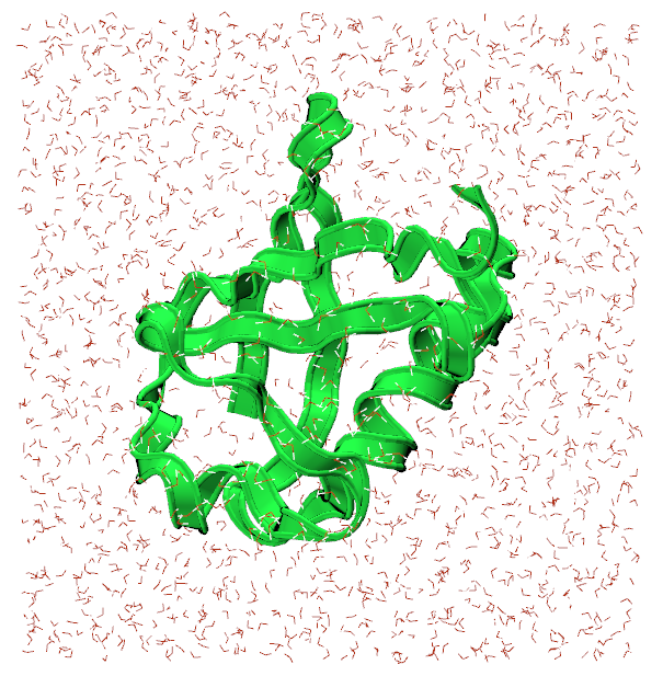
The representation for the protein is set to Ribbons for visibility sake.

In the 1-3-box directory, there is a NAMD configuration file, ubq_wb_eq.conf, that is set to run an equilibration of ubiquitin in water. This is the .conf that we will be running on Thorny Flat.

Transferring files to the HPC

The best way to go about transferring files to the HPC is by using Globus Connect, a service we pay for to transfer files around WVU. There is a wonderful GUI that we can use to access the filesystem on Thorny Flat, and send the necessary files to run the simulation.

Navigate to the Globus homepage and log in with your wvu credentials. This should direct you to the File Manager where the file transferring is done.

For Globus to see the files on your computer, download Globus Connect Personal for your OS. There will be instructions to set up your computer as a Globus Endpoint.

Once complete, there will be an endpoint listed under your collections with the name provided for it:

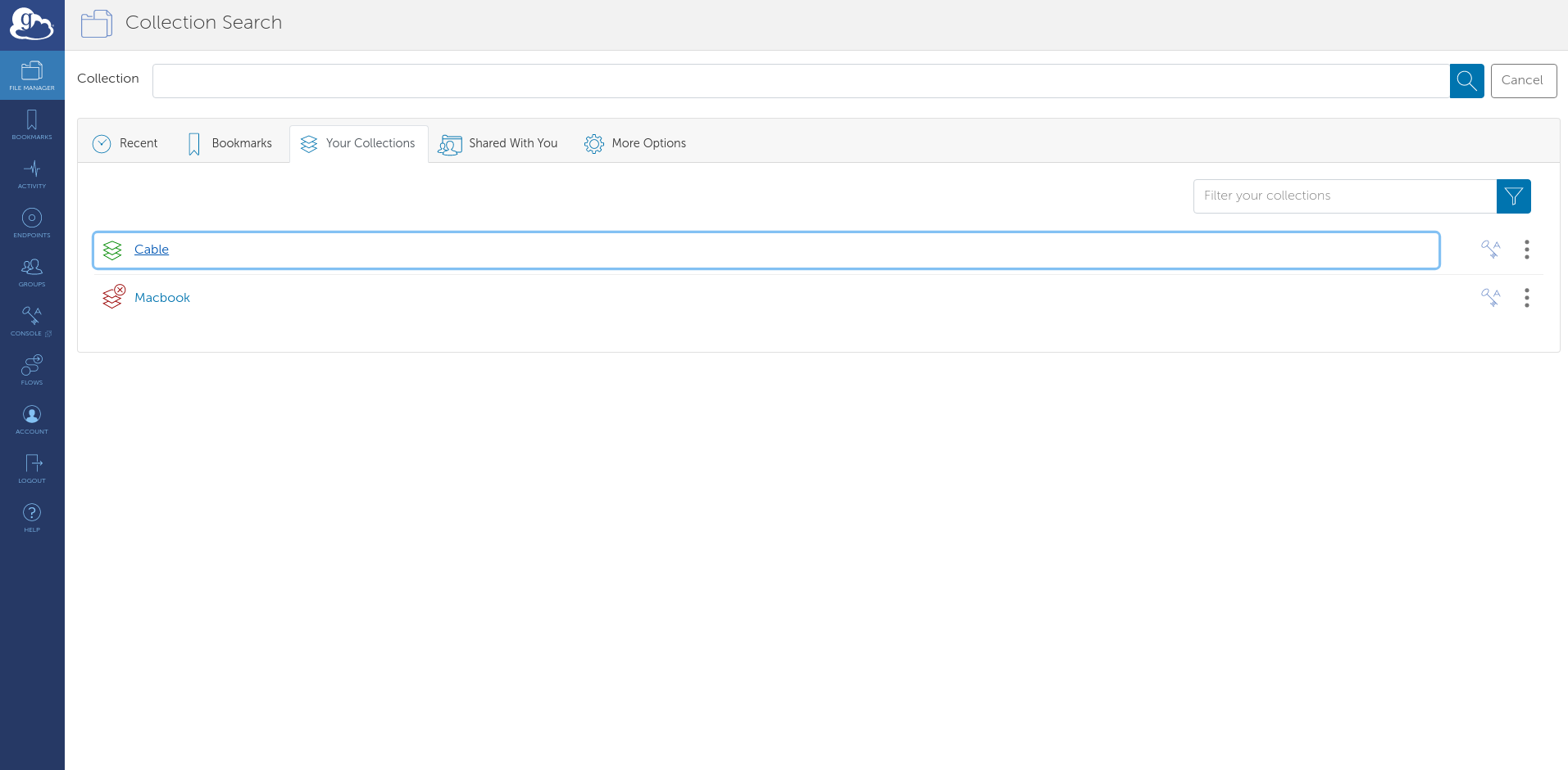
Select it and the files locally available files will appear. Now, select the other side of the File Manager and search for: wvu#thornydtn. This is the name of the endpoint that will allow us to access Thorny Flat.

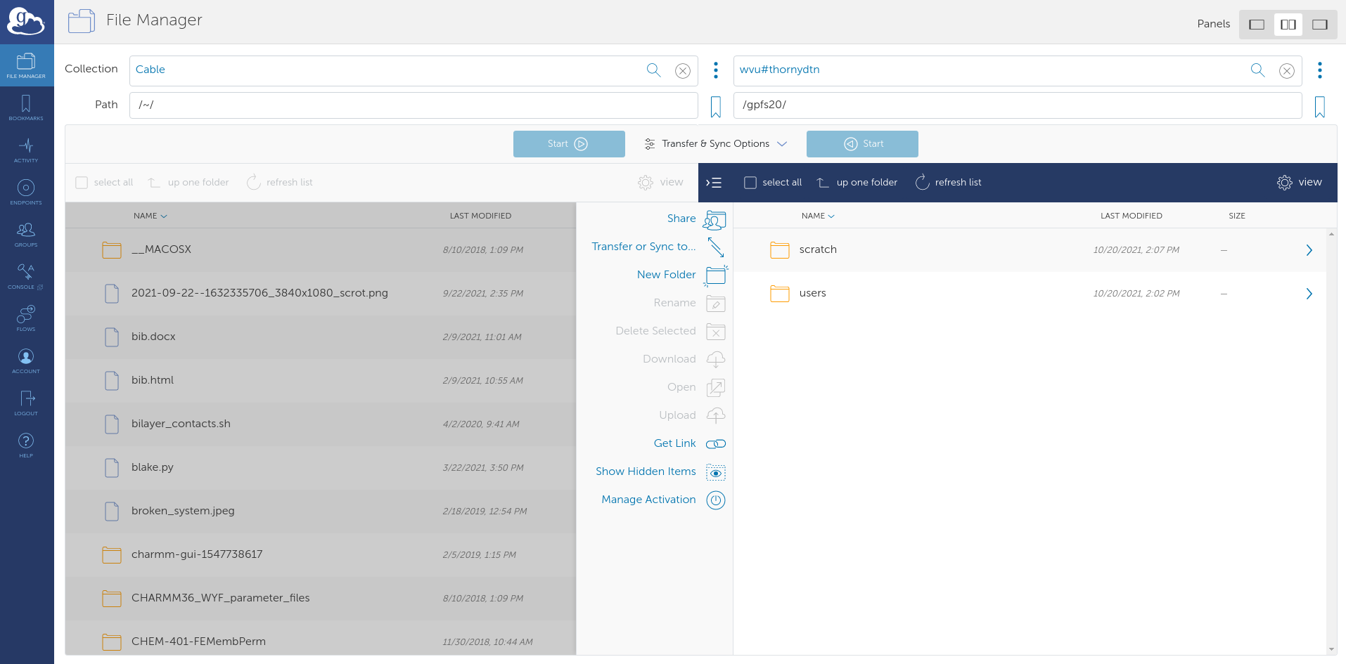
Navigate to to the directory containing the namd_tutorial_files directory in the File Manager and select the namd_tutorial_files directory so it is highlighter blue. Next, on the wvu#thornydtn side, enter the scratch directory and then the directory bearing your wvu username.

Press the blue start button on the left to transfer the files to your scratch directory on Thorny Flat.

Connecting to the cluster

Open OnDemand is an excellent user-friendly way to communicate with the cluster if you don’t have a locally installed terminal.

Navigate to the Thorny Flat OnDemand page and from the drop-down menus at the top select Clusters>Thorny Flat Shell Access. This will open a shell that can be used to talk to the cluster.

Moving around with the command line

Welcome to a command line interface (CLI)! This simple looking tool is capable of running some very powerful, diverse commands, however, you need only a few of them to submit a job to the HPC.

The first command to use is cd to change directory from one to another. This is akin to double-clicking a folder on Windows or Mac.

You want to use cd to move to the directory you transferred over with Globus. To do that, execute:

$ cd $SCRATCH

Shell commands seen here and online often have the leading $. You don’t need to type these in; they’re only there to show that this is a shell command. Press enter to execute the command. The shell won’t output anything, but you should see a change in the line the cursor is on now. The ~ that was there in the previous line has become your username; this represents your current directory. Also the $SCRATCH in the command is a variable that represents the pathway to your scrach directory. Execute the following command to get a better look at where you are:

$ pwd

/scratch/ncf0003/

This command prints the full path of where you presently are. Similar to C:\Users\ncf0003\Documents on Windows.

Now, to see the contents of the directory, execute the command: ls.

namd-tutorial-files

This will output all files and directories contained in the directory.

You can see the namd-tutorial-files directory that you transferred with Globus. Now, execute:

$ cd namd-tutorial-files/1-3-box/

This is the directory where you will run your first job on the HPC!

Making a pbs script and submitting a job

To submit a job to the HPC, you need to make a script called a “pbs script”. This is a list of commands understood by the computer to start running your job. To make your pbs script, execute the following:

$ nano pbs.sh

The nano command makes a new file with the name you gave it, in this case, pbs.sh. It also opens a new window that is mostly blank with commands at the bottom. This is a text editor; think of it like notepad. You should be able to copy-paste the text fromthe box below into the Open OnDemand window.

#!/bin/bash
#PBS -q standby                # queue you're submitting to
#PBS -m ae                     # sends an email when a job ends or has an error
#PBS -M ncf0003@mix.wvu.edu    # your email
#PBS -N ubq_wb_eq              # name of your job; use whatever you'll recognize
#PBS -l nodes=1:ppn=40         # resources being requested; change "node=" to request more nodes
#PBS -l walltime=10:00         # this dictates how long your job can run on the cluster; 7:00:00:00 would be 7 days


# Load the necessary modules to run namd
module load lang/intel/2018 libs/fftw/3.3.9_intel18 parallel/openmpi/3.1.4_intel18_tm

# Move to the directory you submitted the job from
cd $PBS_O_WORKDIR              

# Pathway to the namd2 code
MD_NAMD=/scratch/jbmertz/binaries/NAMD_2.14_Source/Linux-x86_64-icc-smp/

# actual call to run namd
mpirun --map-by ppr:2:node ${MD_NAMD}namd2 +setcpuaffinity +ppn$(($PBS_NUM_PPN/2-1)) ubq_wb_eq.conf > ubq_wb_eq.log

The top block of block of commands that begin with #PBS are specifying how you’d like to run your job on the cluster; you can see a brief description of what they do later in each line. Lets skip the -q line for now and talk about the rest of the #PBS lines. The -m and -M lines are about emailing you confirmation of different things happening to your job; they can be omitted if you would not like to be emailed. -N specifies a name for your job; it will appear when you check your job later on to see its progress. There are two lines of -l that inform the HPC how many compute nodes you need and for how long; these can be restricted by the queue you are trying to use in the first line.

Exit nano for now by pressing Ctrl-X, then Enter to save the script.

Queues

There are severa different queues on the HPC and their names aren’t misnomers; they are lines that your job will wait in for computing time. It can be a little bit of a balancing act to determine which queue will let you use enough resources for enough time while not having to wait too long. First, to see the queues of Thorny Flat, execute:

$ qstat -q

server: trcis002.hpc.wvu.edu
Queue            Memory CPU Time Walltime Node  Run Que Lm  State
---------------- ------ -------- -------- ----  --- --- --  -----
standby            --      --    04:00:00   --   15 136 --   E R
comm_small_week    --      --    168:00:0   --   28 202 --   E R
comm_small_day     --      --    24:00:00   --   21 529 --   E R
comm_gpu_week      --      --    168:00:0   --    8  15 --   E R
comm_xl_week       --      --    168:00:0   --    4   4 --   E R
jaspeir            --      --       --      --    0   0 --   E R
jbmertz            --      --       --      --   19   1 --   E R
vyakkerman         --      --       --      --    1   0 --   E R
bvpopp             --      --       --      --    0   0 --   E R
spdifazio          --      --       --      --    0   0 --   E R
sbs0016            --      --       --      --    0   0 --   E R
pmm0026            --      --       --      --    3   0 --   E R
admin              --      --       --      --    0   0 --   E R
debug              --      --    01:00:00   --    0   0 --   E R
aei0001            --      --       --      --    0   0 --   E R
comm_gpu_inter     --      --    04:00:00   --    0   0 --   E R
phase1             --      --       --      --    0   0 --   E R
zbetienne          --      --       --      --    0   0 --   E R
comm_med_week      --      --    168:00:0   --    5   1 --   E R
comm_med_day       --      --    24:00:00   --    0   1 --   E R
mamclaughlin       --      --       --      --    1   0 --   E R
zbetienne_small    --      --       --      --    0   0 --   E R
zbetienne_large    --      --       --      --    0   0 --   E R
alromero           --      --       --      --    8 287 --   E R
tdmusho            --      --       --      --    0   0 --   E R
cedumitrescu       --      --       --      --    0   0 --   E R
cfb0001            --      --       --      --    0   0 --   E R
chemdept           --      --       --      --    0   0 --   E R
chemdept-gpu       --      --       --      --    0   0 --   E R
be_gpu             --      --       --      --    0   0 --   E R
ngarapat           --      --       --      --    0   0 --   E R
                                               ----- -----
                                                 113  1176

The column on the left is the name of each queue and the other most important column is the walltime. Now, lots of these queues are owned by research groups and therefore you won’t have access to (i.e., jbmertz is Blake Mertz’s queue that he can dictate who can use). However, every user of the cluster has access to any queue that begins with comm, short for community; the names give a little description of what’s unique to them. comm_small_week gives you access to the smallest ammount of RAM a node has and will let you run for a week. Unless you’re crashing due to memory issues, you should only use the comm_small_week, comm_small_day, and standby queues as communnity queues based on how much walltime you need as well as the chemdept queue.

server: trcis002.hpc.wvu.edu
Queue            Memory CPU Time Walltime Node  Run Que Lm  State
---------------- ------ -------- -------- ----  --- --- --  -----
standby            --      --    04:00:00   --   15 136 --   E R
comm_small_week    --      --    168:00:0   --   28 202 --   E R
comm_small_day     --      --    24:00:00   --   21 529 --   E R
chemdept           --      --       --      --    0   0 --   E R

The HPC has a system set up to fairly distribute time among users so even though there’s 202 jobs in queue for the comm_small_week queue, if you haven’t run a job yet this week, you will effectively hop the line and your job will run before others who have used the community queues. Also, nodes are allocated to jobs based on how much walltime they’re asking to use: ask for less walltime and your job will have a better chance to start sooner. Now, a guaranteed way to start your job is by submitting to a non-community queue that has no jobs in queue such as the chemdept queue. You just need to also have access to the queue to take advantage. However, as soon as the chemistry department’s nodes are done on whatever job they were assigned in the mean time, they will start work on your job.

Getting back to your pbs script, you are looking to run on the standby queue since the simulation you’re running is not long, and for the sake of the workshop, you want it to start quickly.

The rest of the pbs

Execute another nano pbs.sh to get back into your pbs script.

#!/bin/bash
#PBS -q standby                # queue you're submitting to
#PBS -m ae                     # sends an email when a job ends or has an error
#PBS -M ncf0003@mix.wvu.edu    # your email
#PBS -N ubq_wb_eq              # name of your job; use whatever you'll recognize
#PBS -l nodes=1:ppn=40         # resources being requested; change "node=" to request more nodes
#PBS -l walltime=10:00         # this dictates how long your job can run on the cluster; 7:00:00:00 would be 7 days


# Load the necessary modules to run namd
module load atomistic/namd/NAMD_Git-2021-10-06-ofi-smp

# Move to the directory you submitted the job from
cd $PBS_O_WORKDIR              

# actual call to run namd
charmrun ++local +p40 namd2 ubq_wb_eq.conf ++ppn4 +setcpuaffinity > ubq_wb_eq.log

Beynd the #PBS lines, there is a line loading modules that are needed to run namd. In this particular situation, the modules will always be the same, however, when using other software on the HPC, there can be many options for different software packages. To view all the modules on the HPC, execute:

$ module avail

This outputs every piece of software installed on the nodes on Thorny Flat; you can make use of any of these languages/codes if you’d like. For running NAMD, the modules already specified in the pbs script are good.

Next is a command you have already used cd to switch directories to where you submit the job; that is what the $PBS_O_WORKDIR stands for. Finally you have the call to run NAMD; its much longer than running it locally, however, you only need to concern yourself with the .conf and .log files. To change the number of nodes, you will have to adjust the +p40 to reflect the number of cores to be used.

With all the parameters set, Ctrl-X then Enter to save the pbs script, and you can submit your job by executing:

$ qsub pbs.sh

This tells Thorny Flat that you’d like to start waiting in line for your job to run.

Checking jobs, benchmarking, and output files

Now that you have a job submitted (and potentially already running), you can execute the following to check on your submitted jobs:

$ qstat -u ncf0003

trcis002.hpc.wvu.edu: 
                                                                                  Req'd       Req'd       Elap
Job ID                  Username    Queue    Jobname          SessID  NDS   TSK   Memory      Time    S   Time
----------------------- ----------- -------- ---------------- ------ ----- ------ --------- --------- - ---------
569147.trcis002.hpc.wv  ncf0003     standby  ubq_wb_eq        208468     1     40       --   00:10:00 R  00:00:01

This gives us lots of useful information about the job you submitted. You can see the parameters you set in the pbs including the job name (Jobname), queue (Queue), number of nodes (NDS), and walltime (Req’d Time) as well as the status of the job (S) and how long it has been running (Elap Time). There are several different statuses your job can have but most common are “in queue” (Q), “running” (R), and “canceled/completed” (C).

Benchmarking simulations

A section of the NAMD .log file (ubq_wb_eq.log for your job here) returns benchmarking information about the system you’re running; this is an estimation of how fast your job is running how you have submitted it. You can access it by executing:

$ grep Benchmark ubq_wb_eq.log

Info: Benchmark time: 38 CPUs 0.00319642 s/step 0.0184978 days/ns 2025.13 MB memory
Info: Benchmark time: 38 CPUs 0.00319819 s/step 0.018508 days/ns 2025.13 MB memory
Info: Benchmark time: 38 CPUs 0.00224249 s/step 0.0129774 days/ns 2025.13 MB memory
Info: Benchmark time: 38 CPUs 0.00239816 s/step 0.0138783 days/ns 2025.13 MB memory
Info: Benchmark time: 38 CPUs 0.00244654 s/step 0.0141582 days/ns 2025.13 MB memory
Info: Benchmark time: 38 CPUs 0.00373922 s/step 0.021639 days/ns 2025.13 MB memory

Conventionally, people use nanoseconds (ns) per day to estimate the best efficiency; you can calculate ns/day by inverting the days/ns column there. For instance, the output above claims you will have 60.20548131 ns/day after averaging those outputs.

To actually produce a curve for benchmarking, you would need to run your job with different numbers of nodes (usually 1, 2, 4, and 8). The plot below is an example of a typical benchmarking curve:

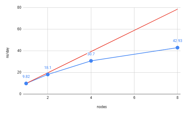
The red line represents perfect scaling based on the simulation using only one node. From there you can see that the actual number of ns/day achieved by the cluster is less than perfect; this is inherent in how the computer functions. This can be plotted another way by looking at how close the simulation is to achieving perfect scaling:

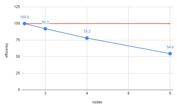
Now, with efficieny on the y-axis, perfect scaling becomes a horizontal line at 100% and you can see how well each number of nodes is performing. Generally, you want ~70% efficieny so you could use 4 nodes in this little example.

Output files

Run another qstat -u ncf0003, and your job is probably done! There are several files created (not just by NAMD) when running a job. Run ls and you should see two files ending in a long string of numbers.

example-output                                            ubq_wb_eq.conf   ubq_wb_eq.coor.BAK  ubq_wb_eq.e569149  ubq_wb_eq.restart.coor      ubq_wb_eq.restart.vel.old  ubq_wb_eq.vel      ubq_wb_eq.xsc.BAK
FFTW_NAMD_2.14_Linux-x86_64-MPI-smp-openmpi-tf_FFTW3.txt  ubq_wb_eq.conf~  ubq_wb_eq.dcd       ubq_wb_eq.log      ubq_wb_eq.restart.coor.old  ubq_wb_eq.restart.xsc      ubq_wb_eq.vel.BAK  ubq_wb_eq.xst
pbs.sh                                                    ubq_wb_eq.coor   ubq_wb_eq.dcd.BAK   ubq_wb_eq.o569149  ubq_wb_eq.restart.vel       ubq_wb_eq.restart.xsc.old  ubq_wb_eq.xsc      ubq_wb_eq.xst.BAK

Here, they are ubq_wb_eq.e569149 and ubq_wb_eq.o569149. These files are the error and output files, respectively, produced by Thorny flat when running your job. Any output produced by your code will go in the output file and same for the error file. These are an excellent first place to look when diagnosing a problem with running on the cluster as they will catch anything that goes wrong with running on the cluster. If you’re however having problems with running NAMD, that will be captured by the NAMD log file (ubq_wb_eq.log for this job) and those should be diagnosed as you would any other simulation.

Visualizing and quick analysis of the trajectory

Now that your simultion should be done (check by executing qstat -u ncf0003), you should transfer the files back to your computer with Globus, this time clicking the transfer button on the right side to send it to your computer.

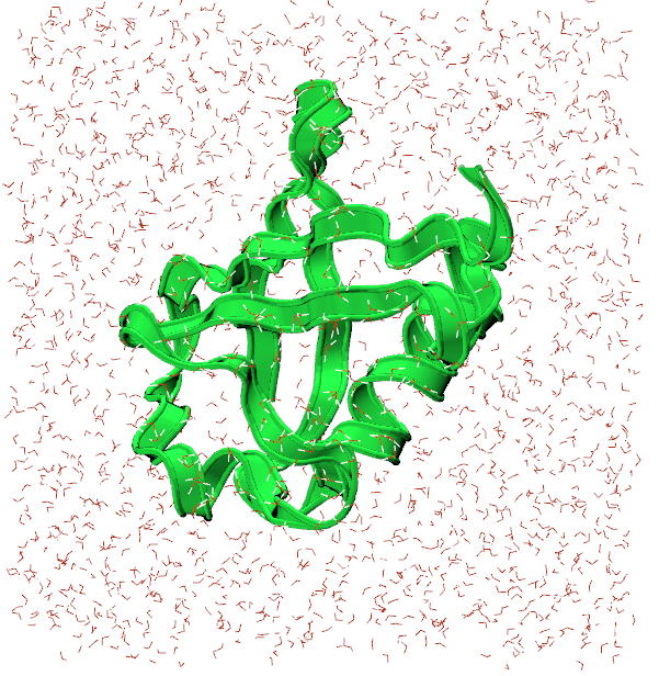
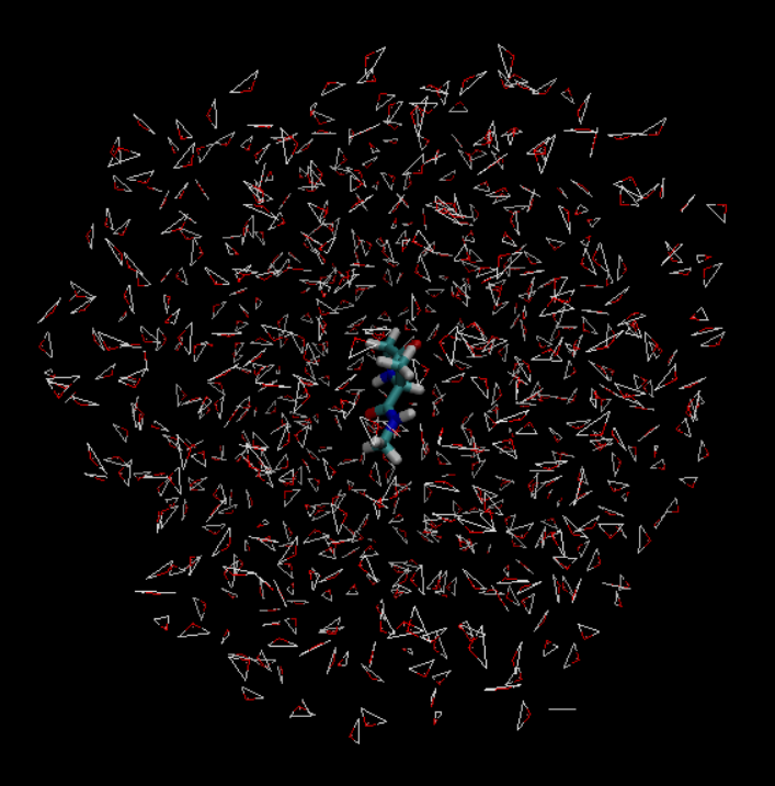
Once the transfer is complete, you can visualize and analyze your trajectory using a tool like VMD again. First, load ubq_wb.psf in to VMD followed by ubq_qb_eq.dcd to visualize your trajectory. Here’s what the final frame could look like:

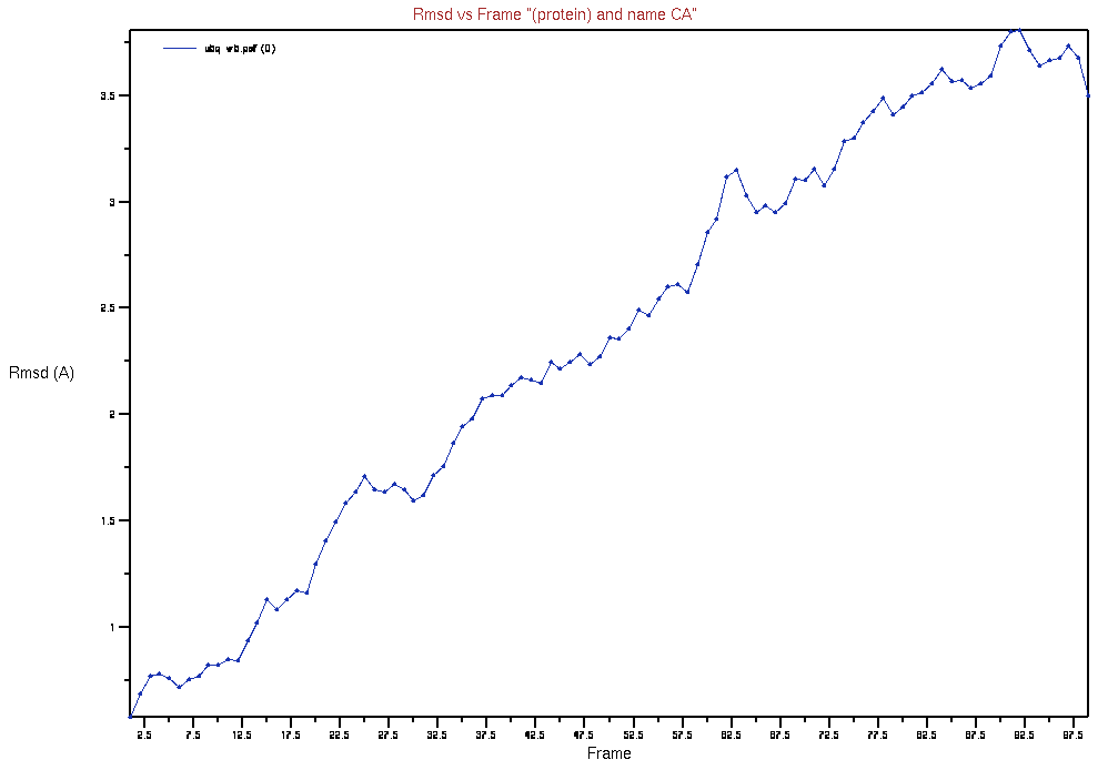
A quick simple bit of analysis could be an RMSD (root-mean-squared deviation) of your system from the initial frame. This will give you a general idea of how much ypur structure changed over the course of the simulation. To do this, navigate to the RMSD Trajectory Tool by going through Extension>Analysis>RMSD Trajectory Tool in the main VMD window. This should open a window similar to the one below:

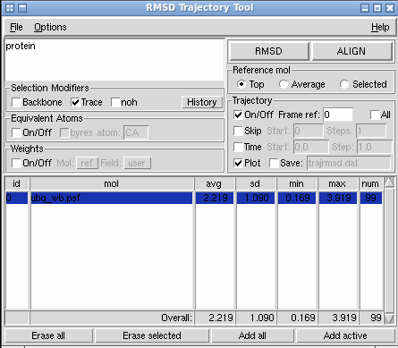
Select “Trace” under “Selection Modifiers” and “Plot” under the “Trajectory” heading. Press the “RMSD” button and, it should produce a plot similar to below:

Key Points

• Globus Connect is the best way to transfer files to the HPC.

• Use a pbs script to submit jobs to the cluster.

• Perform benchmarking to get the most out of your resources.

Using Gromacs on WVU HPC resources

Overview

Teaching: min
Exercises: min

Questions

• What is GROMACS?

• How do I run GROMACS on the cluster?

• How do I check on my job and the simulation status?

Objectives

• Learn about the HPC GROMACS Modules

• Learn how to do some quick analysis on a simulation

“GROMACS”

GROMCS is a free molecular dynamics software package that was originally designed for simulations of biomolecules but, due to it’s high performace and force field options, has also been used in research of non-biological systms such as polymers. It is also user friendly with it’s files and command inputs being easy to understand and use and comes with a full suite of analysis tools.

“GROMACS commands”

All Gromacs commands in current versions start with the binary “gmx” followed by the specific command and inputs such as:

gmx solvate -cp 1AKI_newbox.gro -cs spc216.gro -o 1AKI_solv.gro -p topol.top

This command solvate adds the specified solvent “spc216.gro” into the system provided “1AKI_newbox.gro” and outputs the solvate system as “1AKI_solv.gro” the flags used are uniform across all GROMACS commands to prevent confusion. A full list of all commands and thire use is availble by use of the gmx help option or the online gromacs manuel https://manual.gromacs.org/current/user-guide/cmdline.html

“Lysozyme tutorial”

There are multiple tutorials for gromacs at the website http://www.mdtutorials.com/gmx/index.html the first and simplest is the lysozyme in water that provides a good first time experience with GROMACS with good explanations of each step in introductions to the commonly used files, while the others provide experience in other methods and systems setups of md simulations. The first parts of this tutorial, which consist of the setup and minimization, can be completed in a rather short time frame and it is recommended that you experiment with them to learn more at a later time.

GROMACS_TUTORIAL.zip

The later half of the tutorial is the actual MD simulations and can take a quite a few hours to complete depending on the computer, and this issue just gets worse as the sysems size and complexity increases. This situation is where the HPC’s are extremely useful, allowing the completetion of simulations far faster than what you be possible otherwise. As such these steps will be done on the HPC following the transfer of the files.

cd /scratch/yourdirectory/GROMACS_tutorial

To use the HPC, a pbs script is required, this script contains the modules the HPC has to load, the queue the job is to run on, how long to run the job, the commands to be executed and where they are to be run, amount of nodes requested, the job name, and your email. As long as the pbs script is prepared properly the HPC will queue up the job and run the simulations.

“HPC GROMACS MODULES”

There are multiple GROMACS modules availble on the HPC at WVU allowing for different versions of the software to be used, allowing use of old versions, or use of versions specilized for different software or hardware specifications. The full list of all modules is avalible with the module avail command with the avalible GROMACS versions being in the tier2 modules and all begining with atomistic/gromacs/ and can be loaded with the module load command.

$ module avail

$ module load

“Loading other modules” The GROMACS software can not run by itself and requires other sofware package to be loaded to run and while it is possible to try and run a command with out them the only result would be a line of text informing you the name of the missing module it is far quicker to check before hand the the module show command. This command outputs info about the module specified inculing the modules it depends on.

module show atomistic/gromacs/XXX

“gmx or gmx_mpi”

One of the more common types of avalible GROMACS versions are the MPI versions of GROMACS that are set up to take full advantage of avalible GPUs. These MPI versions of GROMACS do not have the default binary command of gmx but a binary on gmx_mpi, thus it is important to identify which binary is to be used in the command.

The module show command is usefull for identifing these MPI versions as these version require certain other types of module to be loaded such as gcc libaries or openmpi software to be loaded.

“PBSexample”

An example of a pbs script is below just create a file and copy and paste the text into it.

#!/bin/bash

#PBS -q comm_gpu_week
###comm_gpu_week ###standby ###debug
##select which queue to submit to

#PBS -m abe
###send email at (a)bort, (b)egin, (e)nd

#PBS -M YOUR@email.here
###select email to send messages to

#PBS -N jobname
###select jobname

#PBS -l walltime=168:00:00
###walltime in hh:mm:ss

#PBS -l nodes=1:ppn=8:gpus=1
###set number of nodes and processors per node

module load general_intel18
module load lang/gcc/11.1.0
module load libs/fftw/3.3.9_gcc111
module load atomistic/gromacs/5.1.5_intel18
###tell the cluster to load gromacs
###COMMANDS BELOW

### cd /job directory

cd $PBS_O_WORKDIR
###Your gromacs command here

gmx_mpi grompp -f nvt.mdp -c em.gro -r em.gro -p topol.top -o nvt.tpr

gmx_mpi mdrun -deffnm nvt -nb gpu

gmx_mpi grompp -f npt.mdp -c nvt.gro -r nvt.gro -t nvt.cpt -p topol.top -o npt.tpr

gmx_mpi mdrun -deffnm npt -nb gpu

gmx_mpi grompp -f md.mdp -c npt.gro -t npt.cpt -p topol.top -o md_0_1.tpr

gmx_mpi mdrun -deffnm md_0_1 -nb gpu

“Running the job and job status”

While there are interactive jobs for running this simulation we only need one command to have the HPC run the job:

qsub PBSexample

The status of jobs can be checked with the “qstat” command which will give a list of all jobs currently on the HPC, and jobs for specific users can be isolated with the -u flag.

qstat -u username

“Job output and errors”

The HPC will output infomation about the jobs to files based on the job name and job number “jobname.e5282” these files will contain infomation about the job and commands run and any errors that occured.

“Simulation output”

GROMACS will output multiple files that each record different iinformation about the simulation run such as the energy over time and the particle trajectories, however the .log file contains the record of the simulation’s progress and is important to read to understand GROMACS pefromance, as it gives information about the time spent on each type of calculation and overall simulation speed.

     R E A L   C Y C L E   A N D   T I M E   A C C O U N T I N G

On 4 MPI ranks

 Computing:          Num   Num      Call    Wall time         Giga-Cycles
                     Ranks Threads  Count      (s)         total sum    %
-----------------------------------------------------------------------------
 Domain decomp.         4    1       1001       5.961         38.147   0.5
 DD comm. load          4    1        951       0.076          0.489   0.0
 DD comm. bounds        4    1        901       0.127          0.810   0.0
 Neighbor search        4    1       1001      19.563        125.195   1.7
 Comm. coord.           4    1      49000       9.006         57.634   0.8
 Force                  4    1      50001     739.282       4731.188  62.8
 Wait + Comm. F         4    1      50001       7.435         47.581   0.6
 PME mesh               4    1      50001     362.410       2319.321  30.8
 NB X/F buffer ops.     4    1     148001       8.608         55.086   0.7
 Write traj.            4    1        101       0.852          5.455   0.1
 Update                 4    1      50001       7.702         49.290   0.7
 Constraints            4    1      50003       9.691         62.017   0.8
 Comm. energies         4    1       5001       3.759         24.059   0.3
 Rest                                           1.840         11.779   0.2
-----------------------------------------------------------------------------
 Total                                       1176.312       7528.051 100.0
-----------------------------------------------------------------------------
 Breakdown of PME mesh computation
-----------------------------------------------------------------------------
 PME redist. X/F        4    1     100002     172.900       1106.508  14.7
 PME spread             4    1      50001      73.034        467.395   6.2
 PME gather             4    1      50001      50.968        326.180   4.3
 PME 3D-FFT             4    1     100002      39.695        254.034   3.4
 PME 3D-FFT Comm.       4    1     100002      21.577        138.087   1.8
 PME solve Elec         4    1      50001       4.100         26.237   0.3
-----------------------------------------------------------------------------

               Core t (s)   Wall t (s)        (%)
       Time:     4705.206     1176.312      400.0
                 (ns/day)    (hour/ns)
Performance:        7.345        3.267

“Analysis”

There is not much point in doing simulations if you do not collect infomation at the end, through analysis of the system and how it evolved over the course of the simulation. One type of analysis that should always be done is a visual analysis of the system, as it gives you a perspective on the system that graphs and other anaylsis types will not give. Using VMD load the .gro file and the .trr file and then select the atom types you which to view in the represntations window, in this case to examine the protein you can use use the selction “not resname SOL and not resname ION”.

As memtnioned before GROMACS has a full suite of anaylsis tools inculded all of which could be used to perfore analysis on the system being studied, the examples in the lysozyme tutorial are some of the more basic ones that can be used for most simulations but there are specizied analysis command that can be used for specific puropses such as lipid order and polymer properties. One command thet is important to learn how to use is the gmx select command this command selects user specified particles and outputs them into a .ndx file that is used by other commands. For example, createing an .ndx file for the protien. These groups can be specified in the command line with the - select command otherwise the command brings up coomonly used groups for selection.

gmx select -f npt.gro  -s npt.tpr -on PRO.ndx -select 'atomnr 1 to 1960'

gmx select -f npt.gro  -s npt.tpr -on PRO.ndx

Available static index groups:
 Group  0 "System" (33876 atoms)
 Group  1 "Protein" (1960 atoms)
 Group  2 "Protein-H" (1001 atoms)
 Group  3 "C-alpha" (129 atoms)
 Group  4 "Backbone" (387 atoms)
 Group  5 "MainChain" (517 atoms)
 Group  6 "MainChain+Cb" (634 atoms)
 Group  7 "MainChain+H" (646 atoms)
 Group  8 "SideChain" (1314 atoms)
 Group  9 "SideChain-H" (484 atoms)
 Group 10 "Prot-Masses" (1960 atoms)
 Group 11 "non-Protein" (31916 atoms)
 Group 12 "Water" (31908 atoms)
 Group 13 "SOL" (31908 atoms)
 Group 14 "non-Water" (1968 atoms)
 Group 15 "Ion" (8 atoms)
 Group 16 "CL" (8 atoms)
 Group 17 "Water_and_ions" (31916 atoms)
Specify any number of selections for option 'select'
(Selections to analyze):
(one per line, <enter> for status/groups, 'help' for help, Ctrl-D to end)

Key Points

Using AMBER on WVU HPC resources

Overview

Teaching: 0 min
Exercises: 0 min

Questions

• How do I transfer my files to the HPC?

• How do I run NAMD on the cluster?

• How do I check if my job has failed?

Objectives

• Learn which queues to use

• Learn What Modules to use for AMBER

• Learn to call tleap using a config file

• Learn to vizualize the MD simualltion

• Learn how to do some quick analysis on a simulation

The Ground work

We are using the Alanine dipeptide tutorial in AMBER . The first step of which is to use tleap to make the system. This is done using the PBS script below.

#!/bin/bash
#PBS -N tleap_di-ala
#PBS -m abe
#PBS -q standby
#PBS -l nodes=1:ppn=1


module load atomistic/amber/20_gcc93_serial
# we only need to run this on one core so no need to waste resources
cd $PBS_O_WORKDIR
$AMBERHOME/bin/tleap -f make_system.txt
# abmer home is where all the flies for amber are then we find the binary for tleap
# the -f option allows us to run the make_system.txt

This is in the folder named 01_make_system after entering the directory type qsub make_system.pbs in the command line to run the code.

Minimization

Go into the AMBER and then move into the 01_make_system directory. There is the file called make system. Use qsub make_system.pbs This will take about 1min or so to run. If we look into the folder we can see that it produced the pram7 , rst7 and the leap.log files(look in the output file if you did not run the script), and we can load this into VMD so see the peptide in water. To view the simulation we have to load the pram7 as AMBER7 Parm and the rst as AMBER restart. The molecule should look kinda like this.

To get your VMD window to look like this change add a representation to and then change the selection from all to not water. From there we use the licorice .

We run the mininzation next this again for this system type the following in the termial.

cd ../02-min
ls 

the ouput should look like this.

01_Min.in  02-min.pbs  example_run  parm7  rst7

Lets take a look inside of the pbs code used to run the mininmazation

#!/bin/bash
#PBS -N 02_min
#PBS -m abe
#PBS -q standby
#PBS -l nodes=1:ppn=1


module load atomistic/amber/20_gcc93_serial
# we only need to run this on one core so no need to waste resources
cd $PBS_O_WORKDIR
# we will run this on one core and one node with sander because the PME will not work with
# any change of peridoic boundries
 $AMBERHOME/bin/sander -O -i 01_Min.in -o 01_Min.out -p parm7 -c rst7 -r 01_Min.ncrst -inf 01_Min.mdinfo# here is the flagg
# -O : overwirte any files with the same name
#-i : input config 01_Min.in
#-o : the output log of the sim. 01_Min.out
#-p : the parameter file parm7
#-c : the cordiante file rst7
#-r : the file to restart from 01_Min.ncrst
#-inf : The infroamtion file

Heating

The information for benchmarking an amber simualtion can be found in the. We have not yet prodcued a trajectory file yet. The heating file will be the first file which we get do dynamics. After we move to the Heating directory we can type the qsub 03-heat.in . This will heat the system slowly to the final tempature. By doing this the velcoity of all the atoms slowly increase.

Looking at the PBS code for this you will notice that it looks a lot like the for of min.

#!/bin/bash
#PBS -N 03_heat
#PBS -m abe
#PBS -q standby
#PBS -l nodes=1:ppn=1


module load atomistic/amber/20_gcc93_serial
# we only need to run this on one core so no need to waste resources
cd $PBS_O_WORKDIR
# we will run this on one core and one node with sander because the PME will not work with
# any change of peridoic boundries
$AMBERHOME/bin/sander -O -i 02_Heat.in -o 02_Heat.out -p parm7 -c 01_Min.ncrst -r 02_Heat.ncrst -x 02_Heat.nc -inf 02_Heat.mdinfo
# -x : the output trajectory file

looking into the .mdinfo file we will see the preformance.

-----------------------------------------------------------------------------
| Current Timing Info
| -------------------
| Total steps:     10000 | Completed:      2800 ( 28.0%) | Remaining:      7200
|
| Average timings for last     100 steps:
|     Elapsed(s) =       1.60 Per Step(ms) =      15.99
|         ns/day =      10.81   seconds/ns =    7993.30
|
| Average timings for all steps:
|     Elapsed(s) =      44.52 Per Step(ms) =      15.90
|         ns/day =      10.87   seconds/ns =    7950.20
|
| Estimated time remaining:       1.9 minutes.
 ------------------------------------------------------------------------------

The average timing for all steps is what would be used to benchmark the system. For a small system like this running the code on one core is fine , given a larger system it may be better to run with more than one core. For most systems nodes=1:ppn=1 would be fine. The time spent in the heat ,eq ,and production steps have been shortened for time. In a real setting we would have to check if the total energy of the heating converged.

Production

We can finally the final step for the production as in the tutorial this one we will not run for time but take a look at the pbs codes to run the production The frist one is an example of using GPU acceraltion.

#!/bin/bash
#PBS -N 04-production
#PBS -m abe
#PBS -q comm_gpu_week
#PBS -l nodes=1:ppn=1:gpus=1
#PBS -l walltime=10:00:00
module load atomistic/amber/20_gcc93_mpic341_cuda113
cd $PBS_O_WORKDIR
# I have to add the -AllowSmallBox due to the very small size of the system but normally DO NOT
# put this in
$AMBERHOME/bin/pmemd.cuda -AllowSmallBox -O -i 03_Prod.in -o 03_Prod.out -p parm7 -c 02_Heat.ncrst -r 03_Prod.ncrst -x 03_Prod.nc -inf 03_Prod.info

The key difference between this an the other simualtions ran so far is that we are running this with pmemd.cuda instead of sander. We can do that beacuse the system should have by this point have its PBC boundry be stabel and the fluxtions of the box will be small. AMBER is really good at using Cuda cores, and the requried cores #PBS -l nodes=1:ppn=1:gpus=1 will be effeceint for most systems.

When running the pmemd.cuda line here it turns out that the system we use is really to small to be done with GPU acceraltion. We will have to run this using the regular pmemd binary instead.

| ERROR:   max pairlist cutoff must be less than unit cell max sphere radius!

I ran it again with:

#!/bin/bash
#PBS -N 04-production
#PBS -m abe
#PBS -q comm_small_day
#PBS -l nodes=1:ppn=1
module load atomistic/amber/20_gcc93_mpic341
cd $PBS_O_WORKDIR
# put this in
$AMBERHOME/bin/pmemd -O -i 03_Prod.in -o 03_Prod.out -p parm7 -c 02_Heat.ncrst -r 03_Prod.ncrst -x 03_Prod.nc -inf 03_Prod.info
# ther is no cuda on this the pairlist gets to small for pmemd.cuda

When doing the simulation on the GPU the total estimated time to run the producation was only 35 mintues, but when we change over no cuda code the time changed to 18hours. This gose to show how powerful a GPU can be.

NOTE:Amber NetCdf is not able to be loaded in the windows vesrsion of VMD. Due to time learing to use cpptraj is skipped but the manual has tons of good examples and is very well written.

Key Points

• Sander is used for simualtions that require changes in the periodic box

• The GPU code for amber is run on the GPU and needs only one cpu for commincation to run optimally