Supercomputing: Concepts

Last updated on 2025-08-18 | Edit this page

Estimated time: 60 minutes

Overview

Questions

“What is supercomputing?”
“Why I could need a supercomputer?”
“How a supercomputer compares with my desktop or laptop computer?”

Objectives

“Learn the main concepts of supercomputers”
“Learn some use cases that justify using supercomputers.”
“Learn about HPC cluster a major category of supercomputers.”

Introduction

The concept of “supercomputing” refers to the use of powerful computational machines for the purpose of processing massively and complex data or conduct large numerical or symbolic problems using the concentrated computational resources. In many cases supercomputers are build from multiple computer systems that are meant to work togheter in parallel. Supercomputing involves a system working at the maximum potential and whose performance is larger of a normal computer.

Sample use cases include weather, energy, life sciences, and manufacturing.

Software concepts

Processes and threads

Threads and processes are both independent sequences of execution. In most cases the computational task that you want to perform on an HPC cluster runs as a single process that could eventually span across multiple threads. You do not need to have a deep understanding of these two concepts but at least the general differenciation is important for scientific computing.

Process: Instance of a program, with access to its own memory, state and file descriptors (can open and close files)
Thread: Lightweight entity that executes inside a process. Every process has at least one thread and threads within a process can access shared memory.

A first technique that codes use to accelerate execution is via multithreading. Almost all computers today have several CPU cores on each CPU chip. Each core is capable of its own processing meaning that you can from a single process span multiple threads of execution each doing its own portion of the workload. As all those threads execute inside the same process and can see the same memory allocated to the process threads can be organized to divide the workload. The various CPU cores can run different threads and achieve an increase of performance as a result. In scientific computing this kind of parallel computing is often implemented using OpenMP but there are several other mechanisms of multicore execution that can be implemented.

The differences between threads and processes tend to be described in a language intended for computer scientists. See for example the discussion “What is the difference between a process and a thread?”

If the discussion above end up being over technical this resouce “Process vs Thread” address the difference from a more informal perspective.

The use of processes and threads is critical in type of parallelization your code can use and will determine how/where you will run your code. Generally speaking there are three kinds of parallelization:

Distributed-memory applications where multiple processes (instances of a program) can be run on one or more nodes. This is the kind of parallelization used by codes that use the Message Passing Interface (MPI). We will discuss in more detail later in this episode.
Shared-memory or Multithreaded applications use one or more CPU cores but all the processing must happen on a single node. One example of this in scientific computing is the use of OpenMP of OpenACC by some codes.
Hybrid parallelization applications combine distributed and multithreading parallelism so you can achieve the best performance. Different processes can be run on one or more nodes and each process can span multiple threads and use efficiently several CPU cores on the same node. The challenge with this parallelization is the balance between threads and processes as we will discusse later.
Accelerated or GPU-accelerated applications use accelerators such as GPUs that are inherently parallel in nature. Inside this devices multiple threads take place.

Parallel computing paradigms

Parallel computing paradigms can be broadly categorized into shared memory and distributed memory models, with further distinctions within each. These models dictate how processes access and share data. This influencing the design and scope of parallel algorithms.

Shared-Memory

Computeres today have several CPU cores printed inside a single CPU chip and HPC nodes usually have 2 or 4 CPUs and those CPUs can see all the memory installed on the node. All CPU cores sharing all the memory of the node allows for a kind of parallelization where we need to do the same operations to a big pool of data and we can assigned several cores to work on chunks of the data knowing that the results of the operation can be aggregated on the same memory that is visible to all the cores at the end of the procedure.

Multithreading parallelism is the use of several CPU cores by spaning several threads on a single process so data can be processed across the namespace of the process. OpenMP is the de-facto solution for multithreading parallelism. OpenMP is an application programming interface (API) for shared-memory (within a node) parallel programming in C, C++ and Fortran

OpenMP provides a collection of compiler directives, library routines and environment variables.
OpenMP is widely supported by all major compilers, including GCC, Intel, NVIDIA, IBM and AMD Optimizing C/C++ Compiler (AOCC).
OpenMP is portable and can be used one various architectures (Intel, ARM64 and others)
OpenMP is de-facto standard for shared-memory parallelization, there are other options such as Cilk, POSIX threads (pthreads) and specialized libraries for Python, R and other programming languages.

Applications can be parallelized using OpenMP by introducing minor changes to the code in the form of lines that looks like comments and are only interpreted by compilers that support OpenMP. This is a small example

C

#include <omp.h>
#define N 1000
#define CHUNKSIZE 100
main () {
    int i, chunk;
    float a[N], b[N], c[N];
    /* Some initializations */ 
    for (i=0; i < N; i++) a[i] = b[i] = i * 1.0;
    chunk = CHUNKSIZE;

    #pragma omp parallel for \
       shared(a, b, c, chunk) private(i) \
       schedule(static, chunk)
    for (i=0; i < n; i++) c[i] = a[i] + b[i];
}

If you are not a developer what you should know is that OpenMP is a solution to add parallelism to a code and with the right flags during compilation OpenMP can be enabled and the resulting code can work more efficiently on compute nodes.

Message Passing

In the message passing paradigm, each processor runs its own program and works on its own data.

In the message passing paradigm, as each process is independent and has its own memory namespace, different processes need to coordinate the work by sending and receiving messages. Each process must ensure that each it has correct data to compute and write out the results in correct order.

The Message Passing Interface (MPI) is a standard for parallelizing C, C++ and Fortran code to run on distributed memory systems such as HPC clusters. While not officially adopted by any major standards body, it has become the de facto standard (i.e., widely used and several implementations created).

There are multiple open-source implementations, including OpenMPI, MVAPICH, and MPICH along with vendor-supported versions such as Intel MPI.
MPI applications can be run within a shared-memory node. All widely-used MPI implementations are optimized to take advantage of faster intranode communications.
Although MPI is often synonymous with distributed memory parallelization, other options exist such as Charm++, Unified Paralle C, and X10

Example of a code using MPI

FORTRAN

PROGRAM hello_mpi
  INCLUDE 'mpif.h'
  INTEGER :: ierr, my_rank, num_procs

  ! Initialize the MPI environment
  CALL MPI_INIT(ierr)

  ! Get the total number of processes
  CALL MPI_COMM_SIZE(MPI_COMM_WORLD, num_procs, ierr)

  ! Get the rank of the current process
  CALL MPI_COMM_RANK(MPI_COMM_WORLD, my_rank, ierr)

  ! Print the "Hello World" message along with the process rank and total number of processes
  WRITE(*,*) "Hello World from MPI process: ", my_rank, " out of ", num_procs

  ! Finalize the MPI environment
  CALL MPI_FINALIZE(ierr)

END PROGRAM hello_mpi

The exanple above is pretty simple. MPI applications are usually dense and written to be very efficient in their communication. Data is explicitly communicated between processes using point-to-point or collective calls to MPI library routines. If you are not a programmer or application developer, you do not need to know MPI. You should just be aware that it exists, recognize when a code can use MPI for parallelization and that if you are building your executable, use the appropriate wrappers that allow you to create the executable and run the code.

Amdahl’s law and limits on scalability

We start defining speedup as the ratio between the computing time needed by one processor and by N processors.

\[U(N) = \frac{T(1 proc)}{T(N procs)}\]

The speedup is a very general concept and applies to normal life activities. If you need to cut the grass and that take you 1 hour, having someone with a mower can help you and reduce the time to 30 minutes. In that case the speedup is 2. There are always limits to speedup, using the same analogy it is very unlikely that having 60 people with their mowers suceeed in cutting the grass in 1 minute. We will now discuss the limits of scalability from the theoretical point of view and move into more practical considerations.

Amdahl’s law describes the absolute limit on the speedup (A) of a code as a function of the proportion of the code that can be parallelized and the number of processors (CPU cores). This is the most fundamental law of parallel computing!

P is the fraction of the code that run in parallel
S is the fraction of the code that run serial (S = 1– P)
N = number of processors (CPU cores)
A(N) is the speedup as a function of N

\[U(N) = \frac{1}{(1 - P) + \frac{P}{N}}\]

Consider the limit of speedup as the number of processors goes to infinity. This theoretical speedup depends only on the fraction of the code that runs serial

\[\lim_{N \to \infty} U(N) = \lim_{N \to \infty} \frac{1}{(1 - P) + \frac{P}{N}} = \frac{1}{1– P} = \frac{1}{S}\]

Amdahl’s Law demonstrates the theoretical maximum speedup of an overall system and the concept of diminishing returns. Plotted below is the logarithmic parallelization vs linear speedup. If exactly 50% of the work can be parallelized, the best possible speedup is 2 times. If 95% of the work can be parallelized, the best possible speedup is 20 times. According to the law, even with an infinite number of processors, the speedup is constrained by the unparallelizable portion.

Amdahl’s law plot for various values of parallel fraction

Amdahl’s Law is an example of the law of diminishing returns, ie. the decrease in marginal (incremental) output (speedup) of a production process as the amount of a single factor of production is incrementally increased (processors). The law of diminishing returns (also known as the law of diminishing marginal productivity) states that in a productive process, if a factor of production continues to increase, while holding all other production factors constant, at some point a further incremental unit of input will return a lower amount of output.

The Amdahl’s law just sets the theoretical upper limit on speedup, in real-life applications there are other factors that affect scalability. The movement of data often limits even more the scalability. Irregularities of the problem, for example using (non-cartesian grids) or uneven load balance when the the partition of domains leave some processors with less data than most others.

In summary we have this factors limiting scalability

The theoretical Amdahl’s law
Scaling limited by the problem size
Scaling limited by communication overhead
Scaling limited by uneven load balancing

However, HPC clusters are widely used today and some scientific research could not be possible without the use of supercomputers. Most parallel applications do not scale to thousands or even hundreds of cores. Some applications achieve high scalability by the employ several strategies

Grow the problem size with the number of core or nodes (Gustafson’s Law)
Overlap communications with computation
Use dynamic load balancing to assign work to cores as they become idle
Increase the ratio of computation to communications

Weak versus strong scaling

High performance computing has two common notions of scalability. So far we have shown only the scaling fixing the problem size and adding more processors. However, we can also consider the scaling of problems of increasing size by fixing the size per processor. In summary:

Strong scaling is defined as how the solution time varies with the number of processors for a fixed total problem size.
Weak scaling is defined as how the solution time varies with the number of processors for a fixed problem size per processor.

Hardware concepts

Supercomputers and HPC clusters

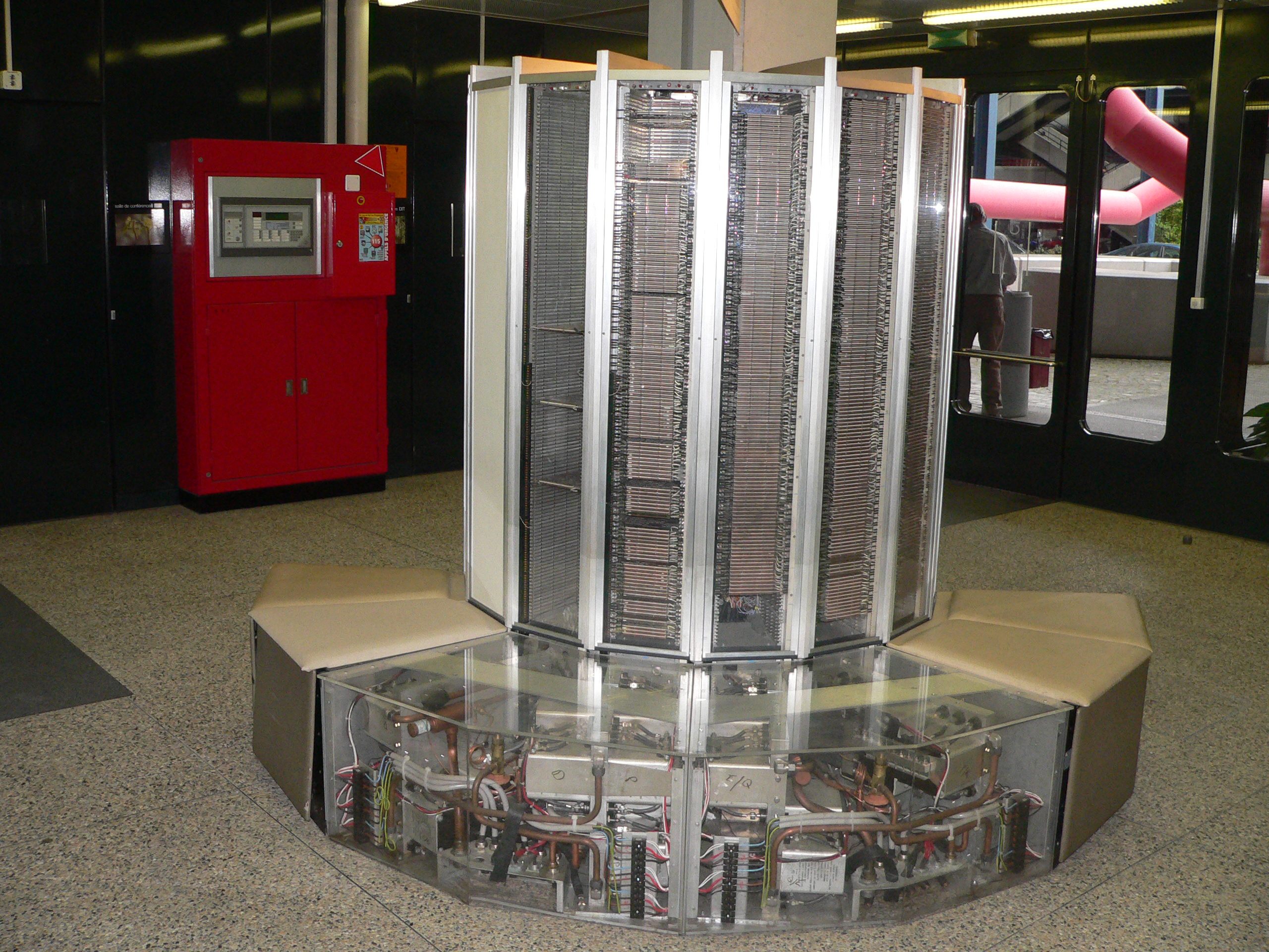
There are many kinds of supercomputers, some of them are build from scratch using specialized hardware, examples of those supercomputers are the iconic CRAY-1 (1976). This machine was the world’s fastest supercomputer from 1976 to 1982. It measured 8½ feet wide by 6½ feet high and contained 60 miles of wires. It achieve a performance of 160 megaflops which is less powerfull than modern smartphones. Many of the CRAY systems from the 80’s and 90’s where machines designed as a single entity using vector processors to achieve their extraordinary performance of their time.

Cray-1 Supercomputer at Bell Labs (Circa-1976)

Modern supercomputers today are usually HPC clusters. HPC clusters consist of multiple compute nodes organized in racks and itnterconnected by one or more networks. Each computer nodes is a computer itself. These aggregates of computers are made to work as a system thanks to sofware that orchestrates their operation and the fast networks that allows data to be moved from one node to another very efficiently.

On each compute node contains one or more (typically two, sometimes four) multicore processors, the CPUs and their internal CPU cores are resposible for the computational capabilities of the node.

Today the computational power comming from CPUs alone is not enough so they receive extra help from other chips in the node specialized in certain computational tasks. These electronic components are called accelerators, among them the GPUs. GPUs are electronic devices that are naturally efficient for certain parallel tasks. They outperform CPUs on a narrow scope of applications. With the current

To effectively use HPC clusters, we need applications that have been parallelized so that they can run on multiple CPU cores. If the calculation is even more demanding even multiple nodes using distributed parallel computing and using GPUs if the algorithm performs efficiently on this kind of acccelerators.

Hierachy of Hardware on an HPC Cluster

At the highest level is the rack. A rack is just a structure to pile up the individual nodes. An HPC cluster can be built from more normal computers but it is often the for the nodes to be rackable, ie, they can be stack on a rack to create a more dense configuration and facilitate administration.

Thorny Flat

Each node on the rack is a computer on itself. Sometimes rack servers are grouped in chassis but often they are just individual machines as shown below.

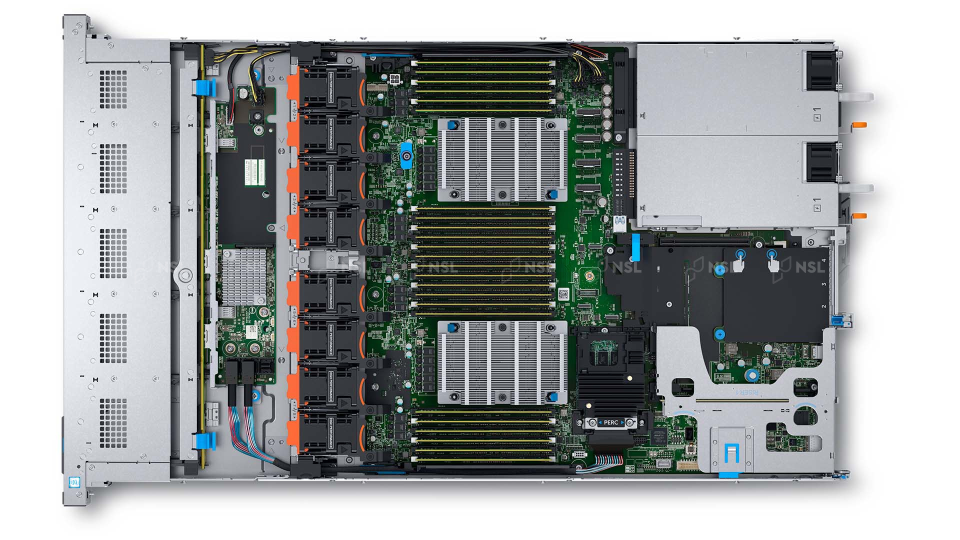
Each compute node has a mainboard, one or more CPUs, RAM modules and network interfaces. They have all that you expect from a computer except for a monitor, keyboard and mouse.

Microprocessor Trends (Performance, Power and Cores)

Microprocessor trends has been collected over the years and can be found on Karl Rupp Github Page

Key Points

“Supercomputers are far more powerful than desktop computers”
“Most supercomputers today are HPC clusters”
“Supercomputers are intended to run large calculations or simulations that takes days or weeks to complete”
“HPC clusters are aggregates of machines that operate as a single entity to provide computational power to many users”