All in One View
Content from Supercomputing: Concepts
Last updated on 2025-08-18 | Edit this page
Overview
Questions
- “What is supercomputing?”
- “Why I could need a supercomputer?”
- “How a supercomputer compares with my desktop or laptop computer?”
Objectives
- “Learn the main concepts of supercomputers”
- “Learn some use cases that justify using supercomputers.”
- “Learn about HPC cluster a major category of supercomputers.”
Introduction
The concept of “supercomputing” refers to the use of powerful computational machines for the purpose of processing massively and complex data or conduct large numerical or symbolic problems using the concentrated computational resources. In many cases supercomputers are build from multiple computer systems that are meant to work togheter in parallel. Supercomputing involves a system working at the maximum potential and whose performance is larger of a normal computer.
Sample use cases include weather, energy, life sciences, and manufacturing.
Software concepts
Processes and threads
Threads and processes are both independent sequences of execution. In most cases the computational task that you want to perform on an HPC cluster runs as a single process that could eventually span across multiple threads. You do not need to have a deep understanding of these two concepts but at least the general differenciation is important for scientific computing.
- Process: Instance of a program, with access to its own memory, state and file descriptors (can open and close files)
- Thread: Lightweight entity that executes inside a process. Every process has at least one thread and threads within a process can access shared memory.
A first technique that codes use to accelerate execution is via multithreading. Almost all computers today have several CPU cores on each CPU chip. Each core is capable of its own processing meaning that you can from a single process span multiple threads of execution each doing its own portion of the workload. As all those threads execute inside the same process and can see the same memory allocated to the process threads can be organized to divide the workload. The various CPU cores can run different threads and achieve an increase of performance as a result. In scientific computing this kind of parallel computing is often implemented using OpenMP but there are several other mechanisms of multicore execution that can be implemented.
The differences between threads and processes tend to be described in a language intended for computer scientists. See for example the discussion “What is the difference between a process and a thread?”
If the discussion above end up being over technical this resouce “Process vs Thread” address the difference from a more informal perspective.
The use of processes and threads is critical in type of parallelization your code can use and will determine how/where you will run your code. Generally speaking there are three kinds of parallelization:
Distributed-memory applications where multiple processes (instances of a program) can be run on one or more nodes. This is the kind of parallelization used by codes that use the Message Passing Interface (MPI). We will discuss in more detail later in this episode.
Shared-memory or Multithreaded applications use one or more CPU cores but all the processing must happen on a single node. One example of this in scientific computing is the use of OpenMP of OpenACC by some codes.
Hybrid parallelization applications combine distributed and multithreading parallelism so you can achieve the best performance. Different processes can be run on one or more nodes and each process can span multiple threads and use efficiently several CPU cores on the same node. The challenge with this parallelization is the balance between threads and processes as we will discusse later.
Accelerated or GPU-accelerated applications use accelerators such as GPUs that are inherently parallel in nature. Inside this devices multiple threads take place.
Parallel computing paradigms
Parallel computing paradigms can be broadly categorized into shared memory and distributed memory models, with further distinctions within each. These models dictate how processes access and share data. This influencing the design and scope of parallel algorithms.
Shared-Memory
Computeres today have several CPU cores printed inside a single CPU chip and HPC nodes usually have 2 or 4 CPUs and those CPUs can see all the memory installed on the node. All CPU cores sharing all the memory of the node allows for a kind of parallelization where we need to do the same operations to a big pool of data and we can assigned several cores to work on chunks of the data knowing that the results of the operation can be aggregated on the same memory that is visible to all the cores at the end of the procedure.
Multithreading parallelism is the use of several CPU cores by spaning several threads on a single process so data can be processed across the namespace of the process. OpenMP is the de-facto solution for multithreading parallelism. OpenMP is an application programming interface (API) for shared-memory (within a node) parallel programming in C, C++ and Fortran
- OpenMP provides a collection of compiler directives, library routines and environment variables.
- OpenMP is widely supported by all major compilers, including GCC, Intel, NVIDIA, IBM and AMD Optimizing C/C++ Compiler (AOCC).
- OpenMP is portable and can be used one various architectures (Intel, ARM64 and others)
- OpenMP is de-facto standard for shared-memory parallelization, there are other options such as Cilk, POSIX threads (pthreads) and specialized libraries for Python, R and other programming languages.
Applications can be parallelized using OpenMP by introducing minor changes to the code in the form of lines that looks like comments and are only interpreted by compilers that support OpenMP. This is a small example
C
#include <omp.h>
#define N 1000
#define CHUNKSIZE 100
main () {
    int i, chunk;
    float a[N], b[N], c[N];
    /* Some initializations */
    for (i=0; i < N; i++) a[i] = b[i] = i * 1.0;
    chunk = CHUNKSIZE;

    #pragma omp parallel for \
       shared(a, b, c, chunk) private(i) \
       schedule(static, chunk)
    for (i=0; i < n; i++) c[i] = a[i] + b[i];
}
If you are not a developer what you should know is that OpenMP is a solution to add parallelism to a code and with the right flags during compilation OpenMP can be enabled and the resulting code can work more efficiently on compute nodes.
Message Passing
In the message passing paradigm, each processor runs its own program and works on its own data.
In the message passing paradigm, as each process is independent and has its own memory namespace, different processes need to coordinate the work by sending and receiving messages. Each process must ensure that each it has correct data to compute and write out the results in correct order.
The Message Passing Interface (MPI) is a standard for parallelizing C, C++ and Fortran code to run on distributed memory systems such as HPC clusters. While not officially adopted by any major standards body, it has become the de facto standard (i.e., widely used and several implementations created).
There are multiple open-source implementations, including OpenMPI, MVAPICH, and MPICH along with vendor-supported versions such as Intel MPI.
MPI applications can be run within a shared-memory node. All widely-used MPI implementations are optimized to take advantage of faster intranode communications.
Although MPI is often synonymous with distributed memory parallelization, other options exist such as Charm++, Unified Paralle C, and X10
Example of a code using MPI
FORTRAN
PROGRAM hello_mpi
  INCLUDE 'mpif.h'
  INTEGER :: ierr, my_rank, num_procs

  ! Initialize the MPI environment
  CALL MPI_INIT(ierr)

  ! Get the total number of processes
  CALL MPI_COMM_SIZE(MPI_COMM_WORLD, num_procs, ierr)

  ! Get the rank of the current process
  CALL MPI_COMM_RANK(MPI_COMM_WORLD, my_rank, ierr)

  ! Print the "Hello World" message along with the process rank and total number of processes
  WRITE(*,*) "Hello World from MPI process: ", my_rank, " out of ", num_procs

  ! Finalize the MPI environment
  CALL MPI_FINALIZE(ierr)

END PROGRAM hello_mpi
The exanple above is pretty simple. MPI applications are usually dense and written to be very efficient in their communication. Data is explicitly communicated between processes using point-to-point or collective calls to MPI library routines. If you are not a programmer or application developer, you do not need to know MPI. You should just be aware that it exists, recognize when a code can use MPI for parallelization and that if you are building your executable, use the appropriate wrappers that allow you to create the executable and run the code.
Amdahl’s law and limits on scalability
We start defining speedup as the ratio between the computing time needed by one processor and by N processors.
\[U(N) = \frac{T(1 proc)}{T(N procs)}\]
The speedup is a very general concept and applies to normal life activities. If you need to cut the grass and that take you 1 hour, having someone with a mower can help you and reduce the time to 30 minutes. In that case the speedup is 2. There are always limits to speedup, using the same analogy it is very unlikely that having 60 people with their mowers suceeed in cutting the grass in 1 minute. We will now discuss the limits of scalability from the theoretical point of view and move into more practical considerations.
Amdahl’s law describes the absolute limit on the speedup (A) of a code as a function of the proportion of the code that can be parallelized and the number of processors (CPU cores). This is the most fundamental law of parallel computing!
- P is the fraction of the code that run in parallel
- S is the fraction of the code that run serial (S = 1– P)
- N = number of processors (CPU cores)
- A(N) is the speedup as a function of N
\[U(N) = \frac{1}{(1 - P) + \frac{P}{N}}\]
Consider the limit of speedup as the number of processors goes to infinity. This theoretical speedup depends only on the fraction of the code that runs serial
\[\lim_{N \to \infty} U(N) = \lim_{N \to \infty} \frac{1}{(1 - P) + \frac{P}{N}} = \frac{1}{1– P} = \frac{1}{S}\]
Amdahl’s Law demonstrates the theoretical maximum speedup of an overall system and the concept of diminishing returns. Plotted below is the logarithmic parallelization vs linear speedup. If exactly 50% of the work can be parallelized, the best possible speedup is 2 times. If 95% of the work can be parallelized, the best possible speedup is 20 times. According to the law, even with an infinite number of processors, the speedup is constrained by the unparallelizable portion.

Amdahl’s Law is an example of the law of diminishing returns, ie. the decrease in marginal (incremental) output (speedup) of a production process as the amount of a single factor of production is incrementally increased (processors). The law of diminishing returns (also known as the law of diminishing marginal productivity) states that in a productive process, if a factor of production continues to increase, while holding all other production factors constant, at some point a further incremental unit of input will return a lower amount of output.
The Amdahl’s law just sets the theoretical upper limit on speedup, in real-life applications there are other factors that affect scalability. The movement of data often limits even more the scalability. Irregularities of the problem, for example using (non-cartesian grids) or uneven load balance when the the partition of domains leave some processors with less data than most others.
In summary we have this factors limiting scalability
- The theoretical Amdahl’s law
- Scaling limited by the problem size
- Scaling limited by communication overhead
- Scaling limited by uneven load balancing
However, HPC clusters are widely used today and some scientific research could not be possible without the use of supercomputers. Most parallel applications do not scale to thousands or even hundreds of cores. Some applications achieve high scalability by the employ several strategies
- Grow the problem size with the number of core or nodes (Gustafson’s Law)
- Overlap communications with computation
- Use dynamic load balancing to assign work to cores as they become idle
- Increase the ratio of computation to communications
Weak versus strong scaling
High performance computing has two common notions of scalability. So far we have shown only the scaling fixing the problem size and adding more processors. However, we can also consider the scaling of problems of increasing size by fixing the size per processor. In summary:
- Strong scaling is defined as how the solution time varies with the number of processors for a fixed total problem size.
- Weak scaling is defined as how the solution time varies with the number of processors for a fixed problem size per processor.
Hardware concepts
Supercomputers and HPC clusters
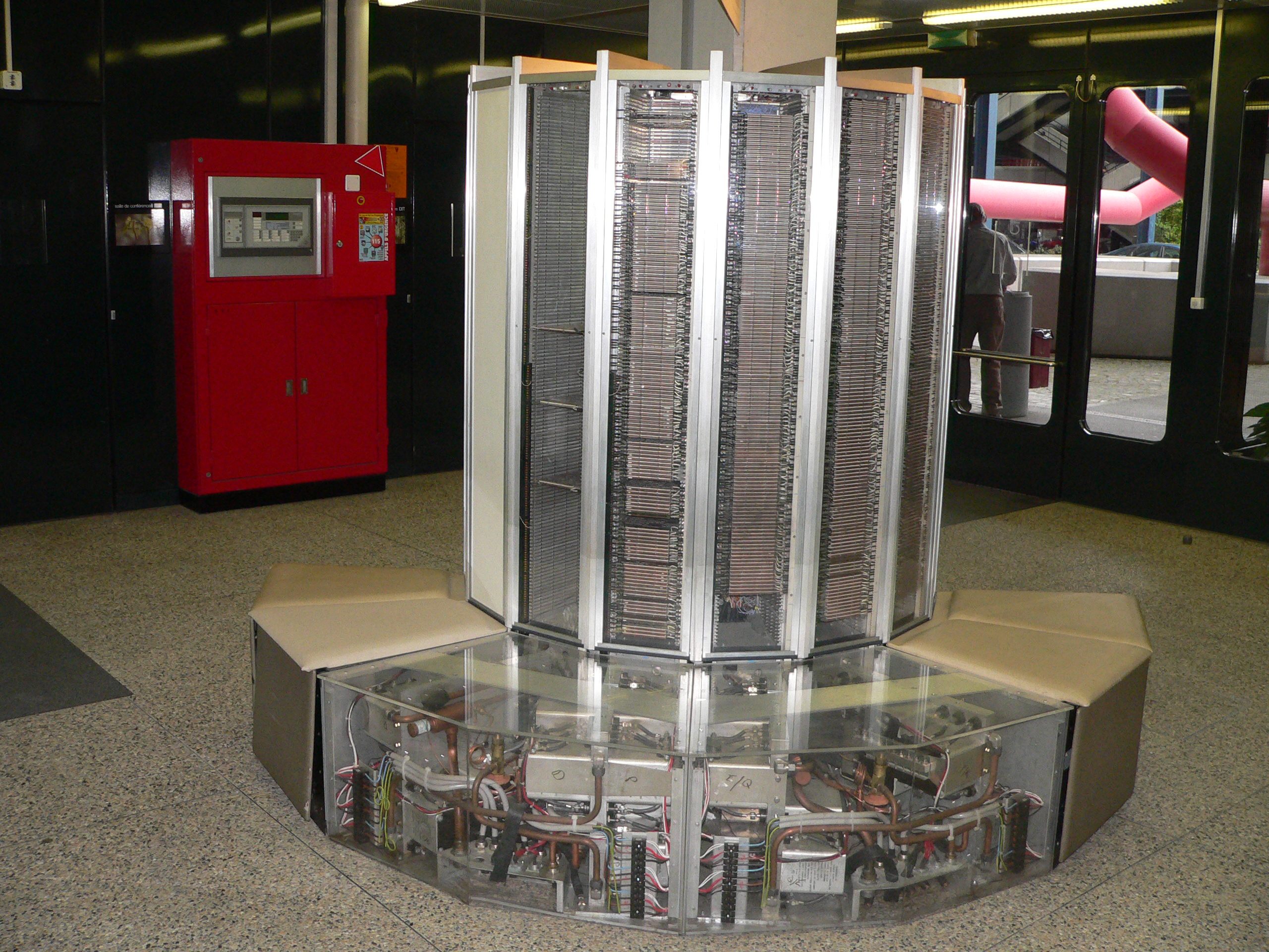
There are many kinds of supercomputers, some of them are build from scratch using specialized hardware, examples of those supercomputers are the iconic CRAY-1 (1976). This machine was the world’s fastest supercomputer from 1976 to 1982. It measured 8½ feet wide by 6½ feet high and contained 60 miles of wires. It achieve a performance of 160 megaflops which is less powerfull than modern smartphones. Many of the CRAY systems from the 80’s and 90’s where machines designed as a single entity using vector processors to achieve their extraordinary performance of their time.
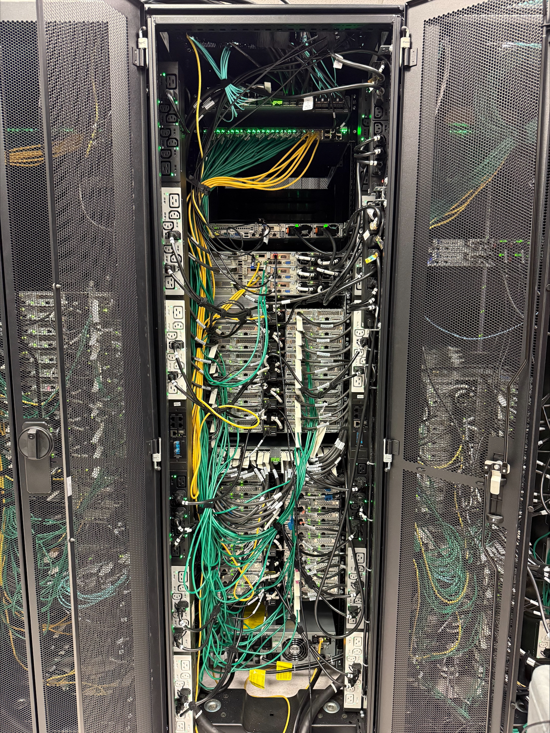
Modern supercomputers today are usually HPC clusters. HPC clusters consist of multiple compute nodes organized in racks and itnterconnected by one or more networks. Each computer nodes is a computer itself. These aggregates of computers are made to work as a system thanks to sofware that orchestrates their operation and the fast networks that allows data to be moved from one node to another very efficiently.

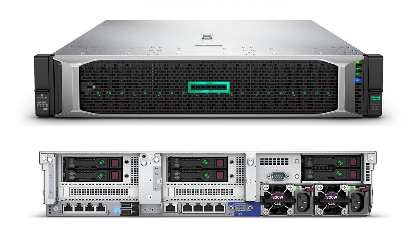
On each compute node contains one or more (typically two, sometimes four) multicore processors, the CPUs and their internal CPU cores are resposible for the computational capabilities of the node.
Today the computational power comming from CPUs alone is not enough so they receive extra help from other chips in the node specialized in certain computational tasks. These electronic components are called accelerators, among them the GPUs. GPUs are electronic devices that are naturally efficient for certain parallel tasks. They outperform CPUs on a narrow scope of applications. With the current
To effectively use HPC clusters, we need applications that have been parallelized so that they can run on multiple CPU cores. If the calculation is even more demanding even multiple nodes using distributed parallel computing and using GPUs if the algorithm performs efficiently on this kind of acccelerators.
Hierachy of Hardware on an HPC Cluster
At the highest level is the rack. A rack is just a structure to pile up the individual nodes. An HPC cluster can be built from more normal computers but it is often the for the nodes to be rackable, ie, they can be stack on a rack to create a more dense configuration and facilitate administration.
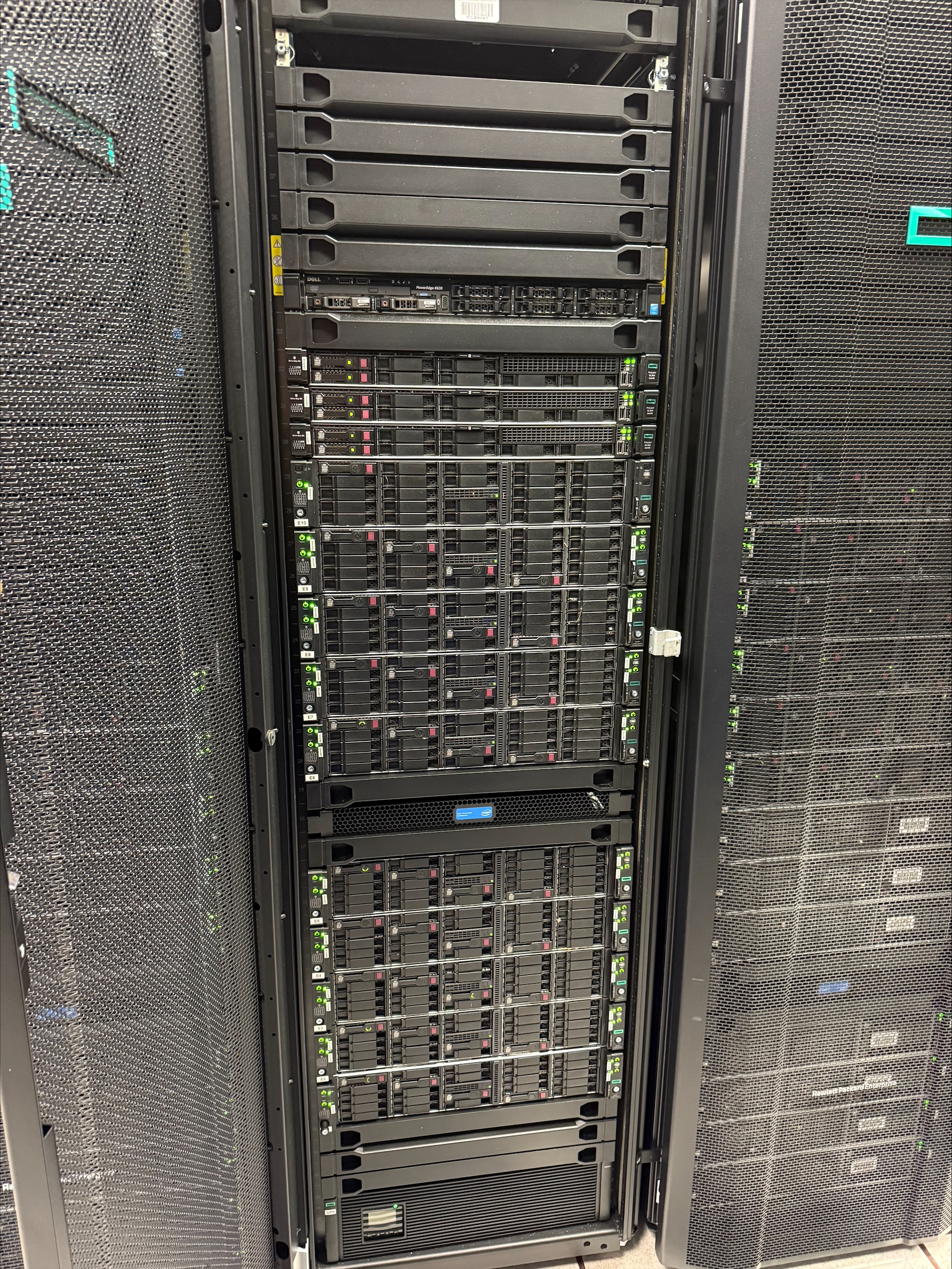
Each node on the rack is a computer on itself. Sometimes rack servers are grouped in chassis but often they are just individual machines as shown below.

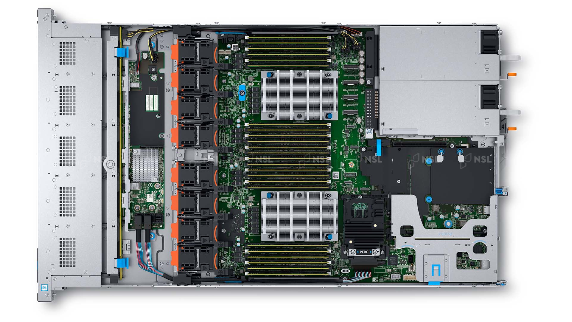
Each compute node has a mainboard, one or more CPUs, RAM modules and network interfaces. They have all that you expect from a computer except for a monitor, keyboard and mouse.
Microprocessor Trends (Performance, Power and Cores)
Microprocessor trends has been collected over the years and can be found on Karl Rupp Github Page

- “Supercomputers are far more powerful than desktop computers”
- “Most supercomputers today are HPC clusters”
- “Supercomputers are intended to run large calculations or simulations that takes days or weeks to complete”
- “HPC clusters are aggregates of machines that operate as a single entity to provide computational power to many users”
Content from The Life Cycle of a Job
Last updated on 2025-08-18 | Edit this page
Overview
Questions
- “Which are the typical steps to execute a job on an HPC cluster?”
- “Why I need to learn commands, edit files and submit jobs?”
Objectives
- “Execute step by step the usual procedure to run jobs on an HPC cluster”
In this episode will will follow some typical steps to execute a calculation using an HPC cluster. The idea is not to learn at this point the commands. Instead the purpose is to provide a reason to why the commands we will learn in future episodes are important to learn and grasp an general perspective of what is involved in using an HPC to carry out research.
We will use a case very specific in Physics, more in particular in Materials Science. We will compute the atomic and electronic structure of Lead in crystalline form. Do not worry about the techical aspects of the particular application, similar procedures apply with small variations in other areas of science: chemistry, bioinformatics, forensics, health sciences and engineering.
Creating a folder for my first job.
The first step is to change our working directory to a location where we can work. Each user has a scratch folder, a folder where you can write files, is visible across all the nodes of the cluster and you have enough space even when large amounts of data are used as inputs or generated as output.
~$ cd $SCRATCHI will create a folder there for my first job and move my working directory inside the newly created folder.
~$ mkdir MY_FIRST_JOB
~$ cd MY_FIRST_JOB
Getting an input file for my simulation
Many scientific codes use the idea of an input file. An input file is just a file or set of files that describe the problem that will be solved and the conditions under which the code should work during the simulation. Users are expected to write their input file, in our case we will take one input file that is ready for execution from one of the examples from a code called ABINIT. ABINIT is a software suite to calculate the optical, mechanical, vibrational, and other observable properties of materials using a technique in applied quantum mechanics called density functional theory. The following command will copy one input file that is ready for execution.
~$ cp /shared/src/ABINIT/abinit-9.8.4/tests/tutorial/Input/tbasepar_1.abi .We can confirm that you have the file in the current folder
~$ ls
tbasepar_1.abi
and get a pick into the content of the file
~$ cat tbasepar_1.abi
#
# Lead crystal
#

#Definition of the unit cell
acell 10.0 10.0 10.0
rprim
    0.0  0.5  0.5
    0.5  0.0  0.5
    0.5  0.5  0.0

#Definition of the atom types and pseudopotentials
ntypat 1
znucl  82
pp_dirpath "$ABI_PSPDIR"
pseudos "Pseudodojo_nc_sr_04_pw_standard_psp8/Pb.psp8"

#Definition of the atoms and atoms positions
natom  1
typat  1
xred
  0.000   0.000   0.000

#Numerical parameters of the calculation : planewave basis set and k point grid
ecut  24.0
ngkpt 12 12 12
nshiftk 4
shiftk
   0.5 0.5 0.5
   0.5 0.0 0.0
   0.0 0.5 0.0
   0.0 0.0 0.5
occopt 7
tsmear 0.01
nband  7

#Parameters for the SCF procedure
nstep   10
tolvrs  1.0d-10

##############################################################
# This section is used only for regression testing of ABINIT #
##############################################################
#%%<BEGIN TEST_INFO>
#%% [setup]
#%% executable = abinit
#%% [files]
#%% files_to_test = tbasepar_1.abo, tolnlines=0, tolabs=0.0, tolrel=0.0
#%% [paral_info]
#%% max_nprocs = 4
#%% [extra_info]
#%% authors = Unknown
#%% keywords = NC
#%% description = Lead crystal. Parallelism over k-points
#%%<END TEST_INFO>
In this example, a single file contains all the input needed. Some other files are used but the input provides instructions to locate those extra files. We are ready to write the submission script
Writing a submission script
A submission script is just a text file that provide information
about the resources needed to carry out the simulation that we pretend
to execute on the cluster. We need to create text file and for that we
will use a terminal-based text editor. The simplest to use is called
nano and for the purpose of this tutorial it is more than
enough.
~$ nano runjob.slurm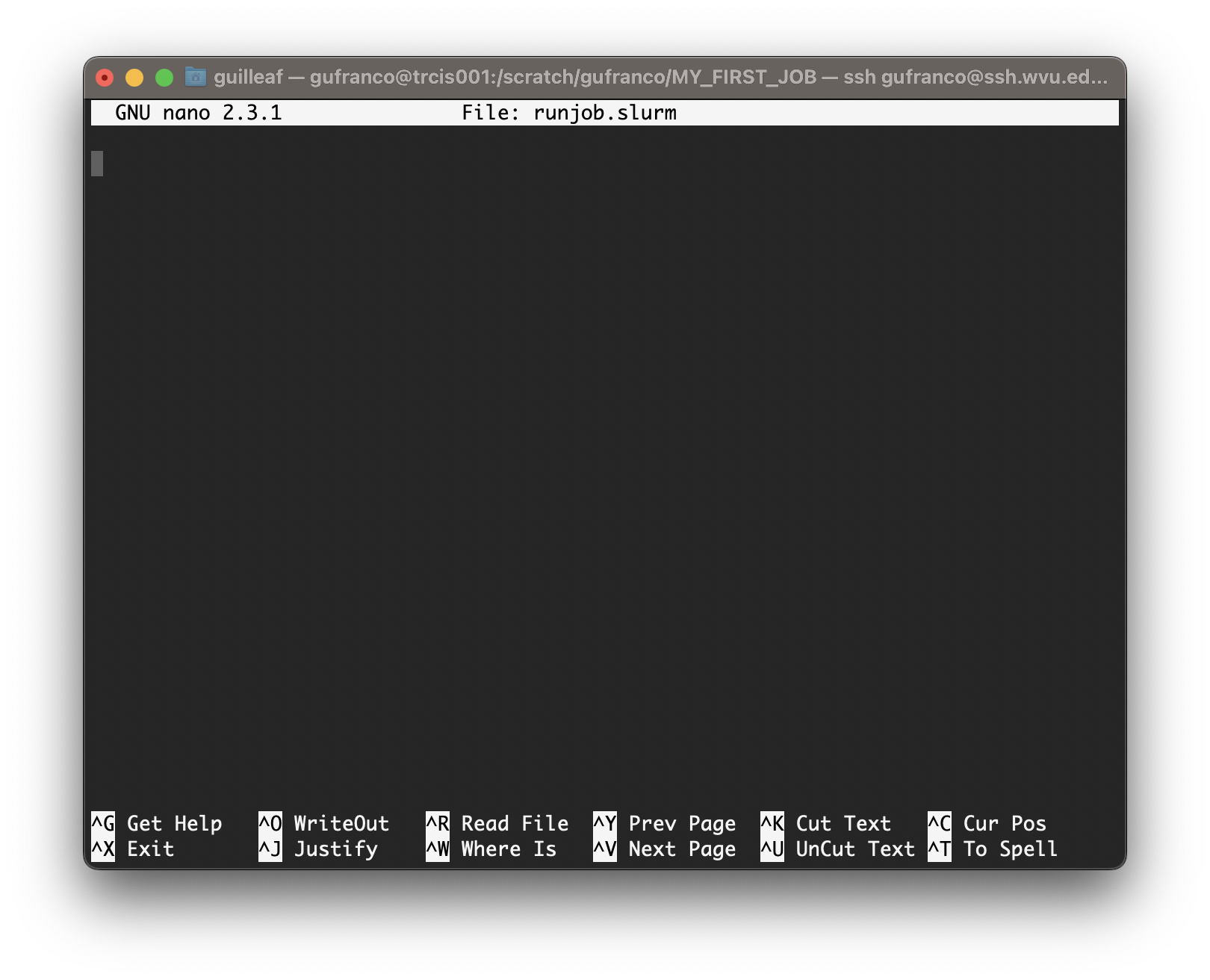
Type the following inside nano window and leave the editor using the command Ctrl+X. Nano will ask if you want to save the changes introduced to the file. Answer with Y It will show the name of your file for confirmation, just click Enter and the file will be saved.
BASH
#!/bin/bash

#SBATCH --job-name=lead
#SBATCH --nodes=1
#SBATCH --cpus-per-task=1
#SBATCH --ntasks=4
#SBATCH --partition=standby
#SBATCH --time=4:00

module purge
module load atomistic/abinit/9.8.4_intel22_impi22

mpirun -np 4 abinit tbasepar_1.abi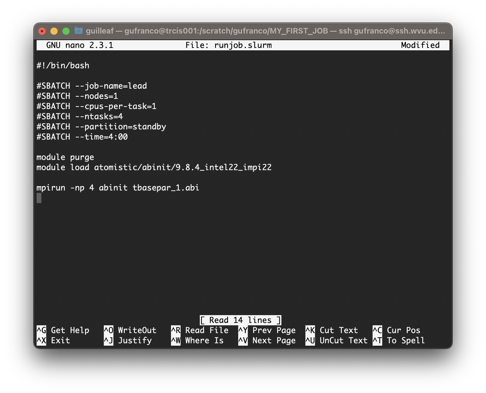
Submitting the job
We use the submission script we just wrote to request the HPC cluster to execute our job when resources on the cluster became available. The job is very small so it is very likely that will execute inmediately. However, in many cases, jobs will remain in the queue for minutes, hours or days depending on the availability of resources on the cluster and the amount of resources requested. Submit the job with this command:
~$ sbatch runjob.slurmYou will get a JOBID number. This is a number that indentify your job. You can check if your job is in queue or executed using the commands
This command to list your jobs on the system:
~$ squeue --meIf the job is in queue or running you can use
~$ scontrol show job <JOBID>If the job already finished use:
~$ sacct -j <JOBID>What we need to learn
The steps above are very typical regardless of the particular code and area of science. As you can see to complete a simulation or any other calculation on an HPC cluster you need.
- Execute some commands. You will learn the basic Linux commands in the next episode.
- Edit some text files. We will present 3 text editors and among them
nano, the editor shown above. - Select a software to run. We are using ABINIT and for it we are using some environment modules to access this software package.
- Submit and monitor jobs on the cluster. All those are Slurm commands and we will learn about them.
In addition to this we will also learn about data transfers to copy files in and out the HPC cluster and tmux, a terminal multiplexer that will facilitate your work on the terminal.
- “To execute jobs on an HPC cluster you need to move across the filesystem, create folders, edit files and submit jobs to the cluster”
- “All these elements will be learned in the following episodes”
Content from Command Line Interface: The Shell
Last updated on 2025-08-27 | Edit this page
Overview
Questions
- “How do I use the Linux terminal?”
Objectives
- “Learn the most basic UNIX/Linux commands”
- “Learn how to navigate the filesystem”
- “Creating, moving, and removing files/directories”
Command Line Interface
At a high level, an HPC cluster is just a bunch of computers that appear to the user like a single entity to execute calculations. A machine where several users can work simultaneously. The users expect to run a variety of scientific codes. To do that, users store the data needed as input, and at the end of the calculations, the data generated as output is also stored or used to create plots and tables via postprocessing tools and scripts. In HPC, compute nodes can communicate with each other very efficiently. For some calculations that are too demanding for a single computer, several computers could work together on a single calculation, eventually sharing information.
Our daily interactions with regular computers like desktop computers and laptops occur via various devices, such as the keyboard and mouse, touch screen interfaces, or the microphone when using speech recognition systems. Today, we are very used to interact with computers graphically, tablets, and phones, the GUI is widely used to interact with them. Everything takes place with graphics. You click on icons, touch buttons, or drag and resize photos with your fingers.
However, in HPC, we need an efficient and still very light way of communicating with the computer that acts as the front door of the cluster, the login node. We use the shell instead of a graphical user interface (GUI) for interacting with the HPC cluster.
In the GUI, we give instructions using a keyboard, mouse, or touchscreen. This way of interacting with a computer is intuitive and very easy to learn but scales very poorly for large streams of instructions, even if they are similar or identical. All that is very convenient but that is now how we use HPC clusters.
Later on in this lesson, we will show how to use Open On-demand, a web service that allows you to run interactive executions on the cluster using a web interface and your browser. For most of this lesson, we will use the Command Line Interface, and you need to familiarize yourself with it.
For example, you need to copy the third line of each of a thousand text files stored in a thousand different folders and paste it into a single file line by line. Using the traditional GUI approach of mouse clicks will take several hours to do this.
This is where we take advantage of the shell - a command-line interface (CLI) to make such repetitive tasks with less effort. It can take a single instruction and repeat it as is or with some modification as many times as we want. The task in the example above can be accomplished in a single line of a few instructions.
The heart of a command-line interface is a read-evaluate-print loop (REPL) so, called because when you type a command and press Return (also known as Enter), the shell reads your command, evaluates (or “executes”) it, prints the output of your command, loops back and waits for you to enter another command. The REPL is essential in how we interact with HPC clusters.
Even if you are using a GUI frontend such as Jupyter or RStudio, REPL is there for us to instruct computers on what to do next.
The Shell
The Shell is a program that runs other programs rather than doing calculations itself. Those programs can be as complicated as climate modeling software and as simple as a program that creates a new directory. The simple programs which are used to perform stand-alone tasks are usually referred to as commands. The most popular Unix shell is Bash (the Bourne Again SHell — so-called because it’s derived from a shell written by Stephen Bourne). Bash is the default shell on most modern implementations of Unix and in most packages that provide Unix-like tools for Windows.
When the shell is first opened, you are presented with a prompt, indicating that the shell is waiting for input.
~$The shell we will use for this lessos will be shown as
~$. Notice that the prompt may be customized by the user to
have more information such as date, user, host, current working
directory and many other pieces of information. For example you can see
my prompt as 22:16:00-gufranco@trcis001:~$.
The prompt
When typing commands from these lessons or other sources, do not type the prompt, only the commands that follow it.
~$ ls -alWhy use the Command Line Interface?
Before the usage of Command Line Interface (CLI), computer interaction took place with perforated cards or even switching cables on a big console. Despite all the years of new technology and innovation, the mouse, touchscreens and voice recognition; the CLI remains one of the most powerful and flexible tools for interacting with computers.
Because it is radically different from a GUI, the CLI can take some effort and time to learn. A GUI presents you with choices to click on. With a CLI, the choices are combinations of commands and parameters, more akin to words in a language than buttons on a screen. Because the options are not presented to you, some vocabulary is necessary in this new “language.” But a small number of commands gets you a long way, and we’ll cover those essential commands below.
Flexibility and automation
The grammar of a shell allows you to combine existing tools into powerful pipelines and handle large volumes of data automatically. Sequences of commands can be written into a script, improving the reproducibility of workflows and allowing you to repeat them easily.
In addition, the command line is often the easiest way to interact with remote machines and supercomputers. Familiarity with the shell is essential to run a variety of specialized tools and resources including high-performance computing systems. As clusters and cloud computing systems become more popular for scientific data crunching, being able to interact with the shell is becoming a necessary skill. We can build on the command-line skills covered here to tackle a wide range of scientific questions and computational challenges.
Starting with the shell
If you still need to download the hands-on materials. This is the perfect opportunity to do so
~$ git clone https://github.com/WVUHPC/workshops_hands-on.gitLet’s look at what is inside the workshops_hands-on
folder and explore it further. First, instead of clicking on the folder
name to open it and look at its contents, we have to change the folder
we are in. When working with any programming tools, folders are
called directories. We will be using folder and directory
interchangeably moving forward.
To look inside the workshops_hands-on directory, we need
to change which directory we are in. To do this, we can use the
cd command, which stands for “change directory”.
~$ cd workshops_hands-onDid you notice a change in your command prompt? The “~” symbol from
before should have been replaced by the string
~/workshops_hands-on$. This means our cd
command ran successfully, and we are now in the new directory.
Let’s see what is in here by listing the contents:
You should see:
Introduction_HPC LICENSE Parallel_Computing README.md Scientific_Programming SparkArguments
Six items are listed when you run ls, but what types of
files are they, or are they directories or files?
To get more information, we can modify the default behavior of
ls with one or more “arguments”.
~$ ls -F

Introduction_HPC/  LICENSE  Parallel_Computing/  README.md  Scientific_Programming/  Spark/
Anything with a “/” after its name is a directory. Things with an asterisk “*” after them are programs. If there are no “decorations” after the name, it’s a regular text file.
You can also use the argument -l to show the directory
contents in a long-listing format that provides a lot more
information:
~$ ls -ltotal 64
drwxr-xr-x 13 gufranco its-rc-thorny 4096 Jul 23 22:50 Introduction_HPC
-rw-r--r-- 1 gufranco its-rc-thorny 35149 Jul 23 22:50 LICENSE
drwxr-xr-x 6 gufranco its-rc-thorny 4096 Jul 23 22:50 Parallel_Computing
-rw-r--r-- 1 gufranco its-rc-thorny 715 Jul 23 22:50 README.md
drwxr-xr-x 9 gufranco its-rc-thorny 4096 Jul 23 22:50 Scientific_Programming
drwxr-xr-x 2 gufranco its-rc-thorny 4096 Jul 23 22:50 SparkEach line of output represents a file or a directory. The directory
lines start with d. If you want to combine the two
arguments -l and -F, you can do so by saying
the following:
~$ ls -lFDo you see the modification in the output?
Details
Notice that the listed directories now have / at the end
of their names.
Tip - All commands are essentially programs that are able to perform specific, commonly-used tasks.
Most commands will take additional arguments controlling their
behavior, and some will take a file or directory name as input. How do
we know what the available arguments that go with a particular command
are? Most commonly used shell commands have a manual available in the
shell. You can access the manual using the man command.
Let’s try this command with ls:
This will open the manual page for ls, and you will lose
the command prompt. It will bring you to a so-called “buffer” page, a
page you can navigate with your mouse, or if you want to use your
keyboard, we have listed some basic keystrokes: * ‘spacebar’ to go
forward * ‘b’ to go backward * Up or down arrows to go forward or
backward, respectively
To get out of the man “buffer” page and to be
able to type commands again on the command prompt, press the
q key!
Exercise
- Open up the manual page for the
findcommand. Skim through some of the information.- Would you be able to learn this much information about many commands by heart?
- Do you think this format of information display is useful for you?
- Quit the
manbuffer (using the keyq) and return to your command prompt.
Tip - Shell commands can get extremely complicated. No one can learn all of these arguments, of course. So you will likely refer to the manual page frequently.
Tip - If the manual page within the Terminal is hard to read and traverse, the manual exists online, too. Use your web-searching powers to get it! In addition to the arguments, you can also find good examples online; Google is your friend.
~$ man findThe Unix directory file structure (a.k.a. where am I?)
Let’s practice moving around a bit. Let’s go into the
Introduction_HPC directory and see what is there.
Great, we have traversed some sub-directories, but where are we in
the context of our pre-designated “home” directory containing the
workshops_hands-on directory?!
The “root” directory!
Like on any computer you have used before, the file structure within a Unix/Linux system is hierarchical, like an upside-down tree with the “/” directory, called “root” as the starting point of this tree-like structure:
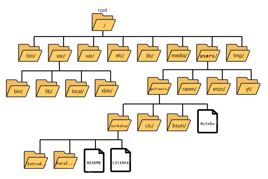
Tip - Yes, the root folder’s actual name is just
/(a forward slash).
That / or root is the ‘top’ level.
When you log in to a remote computer, you land on one of the branches
of that tree, i.e., your pre-designated “home” directory that usually
has your login name as its name (e.g. /users/gufranco).
Tip - On macOS, which is a UNIX-based OS, the root level is also “/”.
Tip - On a Windows OS, it is drive-specific; “C:" is considered the default root, but it changes to”D:", if you are on another drive.
Paths
Now let’s learn more about the “addresses” of directories, called “path”, and move around the file system.
Let’s check to see what directory we are in. The command prompt tells
us which directory we are in, but it doesn’t give information about
where the Introduction_HPC directory is with respect to our
“home” directory or the / directory.
The command to check our current location is pwd. This
command does not take any arguments, and it returns the path or address
of your present working
directory (the folder you are in currently).
~$ pwdIn the output here, each folder is separated from its “parent” or
“child” folder by a “/”, and the output starts with the root
/ directory. So, you are now able to determine the location
of Introduction_HPC directory relative to the root
directory!
But which is your pre-designated home folder? No matter where you
have navigated to in the file system, just typing in cd
will bring you to your home directory.
~$ cdWhat is your present working directory now?
~$ pwdThis should now display a shorter string of directories starting with root. This is the full address to your home directory, also referred to as “full path”. The “full” here refers to the fact that the path starts with the root, which means you know which branch of the tree you are on in reference to the root.
Challenge
Take a look at your command prompt now. Does it show you the name of this directory (your username?)?
No, it doesn’t. Instead of the directory name, it shows you a
~.
Challenge
Why is not showing the path to my home folder?
This is because ~ is a synonimous to the full path to
the home directory for the user.*
Challenge
Can I just type ~ instead of
/users/username?
Yes, it is possible to use ~ as replacement of the full
path to your home folder. You can for example execute:
~$ ls ~~$ cd ~But in this case, it is simpler to just execute
~$ cdTo go to your home folder. There is also a variable called
$HOME that contains the path to your home folder.
Using paths with commands
You can do much more with the idea of stringing together
parent/child directories. Let’s say we want to look at the
contents of the Introduction_HPC folder but do it from our
current directory (the home directory. We can use the list command and
follow it up with the path to the folder we want to list!
~$ cd

~$ ls -l ~/workshops_hands-on/Introduction_HPC
Now, what if we wanted to change directories from ~
(home) to Introduction_HPC in a single step?
Done! You have moved two levels of directories in one command.
What if we want to move back up and out of the
Introduction_HPC directory? Can we just type
cd workshops_hands-on? Try it and see what happens.
Unfortunately, that won’t work because when you say
cd workshops_hands-on, shell is looking for a folder called
workshops_hands-on within your current directory,
i.e. Introduction_HPC.
Can you think of an alternative?
You can use the full path to workshops_hands-on!
Tip What if we want to navigate to the previous folder but can’t quite remember the full or relative path, or want to get there quickly without typing a lot? In this case, we can use
cd -. When-is used in this context it is referring to a special variable called$OLDPWDthat is stored without our having to assign it anything. We’ll learn more about variables in a future lesson, but for now you can see how this command works. Try typing:This command will move you to the last folder you were in before your current location, then display where you now are! If you followed the steps up until this point it will have moved you to
~/workshops_hands-on/Introduction_HPC. You can use this command again to get back to where you were before (~/workshops_hands-on) to move on to the Exercises.
Exercises
- First, move to your home directory.
- Then, list the contents of the
Parallel_Computingdirectory within theworkshops_hands-ondirectory.
Tab completion
Typing out full directory names can be time-consuming and
error-prone. One way to avoid that is to use tab
completion. The tab key is located on the left
side of your keyboard, right above the caps lock key. When
you start typing out the first few characters of a directory name, then
hit the tab key, Shell will try to fill in the rest of the
directory name.
For example, first type cd to get back to your home
directly, then type cd uni, followed by pressing the
tab key:
The shell will fill in the rest of the directory name for
workshops_hands-on.
Now, let’s go into Introduction_HPC, then type
ls 1, followed by pressing the tab key
once:
Nothing happens!!
The reason is that there are multiple files in the
Introduction_HPC directory that start with 1.
As a result, shell needs to know which one to fill in. When you hit
tab a second time again, the shell will then list all the
possible choices.
Now you can select the one you are interested in listed, enter the number, and hit the tab again to fill in the complete name of the file.
NOTE: Tab completion can also fill in the names of commands. For example, enter
e<tab><tab>. You will see the name of every command that starts with ane. One of those isecho. If you enterech<tab>, you will see that tab completion works.
Tab completion is your friend! It helps prevent spelling mistakes and speeds up the process of typing in the full command. We encourage you to use this when working on the command line.
Relative paths
We have talked about full paths so far, but there is
a way to specify paths to folders and files without having to worry
about the root directory. You used this before when we were learning
about the cd command.
Let’s change directories back to our home directory and once more
change directories from ~ (home) to
Introduction_HPC in a single step. (Feel free to use
your tab-completion to complete your path!)
This time we are not using the ~/ before
workshops_hands-on. In this case, we are using a relative
path, relative to our current location - wherein we know that
workshops_hands-on is a child folder in our home folder,
and the Introduction_HPC folder is within
workshops_hands-on.
Previously, we had used the following:
There is also a handy shortcut for the relative path to a parent
directory, two periods ... Let’s say we wanted to move from
the Introduction_HPC folder to its parent folder.
You should now be in the workshops_hands-on directory
(check the command prompt or run pwd).
You will learn more about the
..shortcut later. Can you think of an example when this shortcut to the parent directory won’t work?Answer
When you are at the root directory, since there is no parent to the root directory!
When using relative paths, you might need to check what the branches
are downstream of the folder you are in. There is a really handy command
(tree) that can help you see the structure of any
directory.
If you are aware of the directory structure, you can string together a list of directories as long as you like using either relative or full paths.
Synopsis of Full versus Relative paths
A full path always starts with a /, a relative
path does not.
A relative path is like getting directions from someone on the street. They tell you to “go right at the Stop sign, and then turn left on Main Street”. That works great if you’re standing there together, but not so well if you’re trying to tell someone how to get there from another country. A full path is like GPS coordinates. It tells you exactly where something is, no matter where you are right now.
You can usually use either a full path or a relative path depending on what is most convenient. If we are in the home directory, it is more convenient to just enter the relative path since it involves less typing.
Over time, it will become easier for you to keep a mental note of the structure of the directories that you are using and how to quickly navigate among them.
Copying, creating, moving, and removing data
Now we can move around within the directory structure using the command line. But what if we want to do things like copy files or move them from one directory to another, rename them?
Let’s move into the Introduction_HPC directory, which
contains some more folders and files:
cp: Copying files and folders
Let’s use the copy (cp) command to make a copy of one of
the files in this folder, Mov10_oe_1.subset.fq, and call
the copied file Mov10_oe_1.subset-copy.fq. The copy command
has the following syntax:
cp path/to/item-being-copied path/to/new-copied-item
In this case the files are in our current directory, so we just have to specify the name of the file being copied, followed by whatever we want to call the newly copied file.
The copy command can also be used for copying over whole directories,
but the -r argument has to be added after the
cp command. The -r stands for “recursively
copy everything from the directory and its sub-directories”.
We used it earlier when we copied over the
workshops_hands-on directory to our home directories
#copying-example-data-folder).
mkdir: Creating folders
Next, let’s create a directory called ABINIT and we can
move the copy of the input files into that directory.
The mkdir command is used to make a directory, syntax:
mkdir name-of-folder-to-be-created.
Tip - File/directory/program names with spaces in them do not work well in Unix. Use characters like hyphens or underscores instead. Using underscores instead of spaces is called “snake_case”. Alternatively, some people choose to skip spaces and rather just capitalize the first letter of each new word (i.e. MyNewFile). This alternative technique is called “CamelCase”.
mv: Moving files and folders
We can now move our copied input files into the new directory. We can
move files around using the move command, mv, syntax:
mv path/to/item-being-moved path/to/destination
In this case, we can use relative paths and just type the name of the file and folder.
Let’s check if the move command worked like we wanted:
Let us run abinit, this is a quick execution, and you have not yet learned how to submit jobs. So, for this exceptional time, we will execute this on the login node
mv: Renaming files and folders
The mv command has a second functionality, it is what
you would use to rename files, too. The syntax is identical to when we
used mv for moving, but this time instead of giving a
directory as its destination, we just give a new name as its
destination.
The files t17.out can be renamed, the ABINIT could run again with some change in the input. We want to rename that file:
Tip - You can use
mvto move a file and rename it simultaneously!
Important notes about mv: * When using
mv, the shell will not ask if you are sure
that you want to “replace existing file” or similar unless you use the
-i option. * Once replaced, it is not possible to get the replaced file
back!
Removing
We did not need to create a backup of our output as we noticed this
file is no longer needed; in the interest of saving space on the
cluster, we want to delete the contents of the
t17.backup.out.
Important notes about rm * rm permanently
removes/deletes the file/folder. * There is no concept of “Trash” or
“Recycle Bin” on the command line. When you use rm to
remove/delete, they’re really gone. * Be careful with this
command! * You can use the -i argument if you want
it to ask before removing rm -i file-name.
Let’s delete the ABINIT folder too. First, we’ll have to navigate our way to the parent directory (we can’t delete the folder we are currently in/using).
Did that work? Did you get an error?
Explanation
By default, rm, will NOT delete directories, but you use
the -r flag if you are sure that you want to delete the
directories and everything within them. To be safe, let’s use it with
the -i flag.
-
-r: recursive, commonly used as an option when working with directories, e.g. withcp. -
-i: prompt before every removal.
Exercise
- Create a new folder in
workshops_hands-oncalledabinit_test - Copy over the abinit inputs from
2._Command_Line_Interfaceto the~/workshops_hands-on/Introduction_HPC/2._Command_Line_Interface/abinit_testfolder - Rename the
abinit_testfolder and call itexercise1
Exiting from the cluster
To close the interactive session on the cluster and disconnect from
the cluster, the command is exit. So, you are going to have
to run the exit command twice.
00:11:05-gufranco@trcis001:~$ exit
logout
Connection to trcis001 closed.
guilleaf@MacBook-Pro-15in-2015 ~ %
10 Unix/Linux commands to learn and use
The echo and cat commands
The echo command is very basic; it returns what you give
back to the terminal, kinda like an echo. Execute the command below.
~$ echo "I am learning UNIX Commands"OUTPUT
I am learning UNIX CommandsThis may not seem that useful right now. However, echo
will also print the contents of a variable to the terminal. There are
some default variables set for each user on the HPCs: $HOME
is the pathway to the user’s “home” directory, and $SCRATCH
is Similarly the pathway to the user’s “scratch” directory. More info on
what those directories are for later, but for now, we can print them to
the terminal using the echo command.
~$ echo $HOMEOUTPUT
/users/<username>~$ echo $SCRATCHOUTPUT
/scratch/<username>In addition, the shell can do basic arithmetical operations, execute this command:
~$ echo $((23+45*2))OUTPUT
113Notice that, as customary in mathematics, products take precedence over addition. That is called the PEMDAS order of operations, ie "Parentheses, Exponents, Multiplication and Division, and Addition and Subtraction". Check your understanding of the PEMDAS rule with this command:
~$ echo $(((1+2**3*(4+5)-7)/2+9))OUTPUT
42Notice that the exponential operation is expressed with the
** operator. The usage of echo is important.
Otherwise, if you execute the command without echo, the
shell will do the operation and will try to execute a command called
42 that does not exist on the system. Try by yourself:
~$ $(((1+2**3*(4+5)-7)/2+9))OUTPUT
-bash: 42: command not foundAs you have seen before, when you execute a command on the terminal, in most cases you see the output printed on the screen. The next thing to learn is how to redirect the output of a command into a file. It will be very important to submit jobs later and control where and how the output is produced. Execute the following command:
~$ echo "I am learning UNIX Commands." > report.logWith the character > redirects the output from
echo into a file called report.log. No output is
printed on the screen. If the file does not exist, it will be created.
If the file existed previously, it was erased, and only the new contents
were stored. In fact, > can be used to redirect the
output of any command to a file!
To check that the file actually contains the line produced by
echo, execute:
~$ cat report.logOUTPUT
I am learning UNIX Commands.The cat (concatenate) command displays the contents of one or several files. In the case of multiple files, the files are printed in the order they are described in the command line, concatenating the output as per the name of the command.
In fact, there are hundreds of commands, most of them with a variety of options that change the behavior of the original command. You can feel bewildered at first by a large number of existing commands, but most of the time, you will be using a very small number of them. Learning those will speed up your learning curve.
pwd, cd, and mkdir: Folder
commands
As mentioned, UNIX organizes data in storage devices as a tree. The
commands pwd, cd and mkdir will
allow you to know where you are, move your location on the tree, and
create new folders. Later, we will learn how to move folders from one
location on the tree to another.
The first command is pwd. Just execute the command on
the terminal:
~$ pwdOUTPUT
/users/<username>It is always very important to know where in the tree you are. Doing research usually involves dealing with a large amount of data, and exploring several parameters or physical conditions. Therefore, organizing the filesystem is key.
When you log into a cluster, by default, you are located on your
$HOME folder. That is why the pwd command
should return that location in the first instance.
The following command cd is used to change the
directory. A directory is another name for folder and is
widely used; in UNIX, the terms are interchangeable. Other Desktop
Operating Systems like Windows and MacOS have the concept of smart
folders or virtual folders, where the folder that
you see on screen has no correlation with a directory in the filesystem.
In those cases, the distinction is relevant.
There is another important folder defined in our clusters, it’s
called the scratch folder, and each user has its own. The location of
the folder is stored in the variable $SCRATCH. Notice that
this is internal convection and is not observed in other HPC
clusters.
Use the next command to go to that folder:
~$ cd $SCRATCH
~$ pwd
OUTPUT
/scratch/<username>Notice that the location is different now; if you are using this account for the first time, you will not have files on this folder. It is time to learn another command to list the contents of a folder, execute:
~$ lsAssuming that you are using your HPC account for the first time, you
will not have anything in your $SCRATCH folder and should
therefore see no output from ls. This is a good opportunity
to start your filesystem by creating one folder and moving into it,
execute:
~$ mkdir test_folder
~$ cd test_folder
mkdir allows you to create folders in places where you
are authorized to do so, such as your $HOME and
$SCRATCH folders. Try this command:
~$ mkdir /test_folderOUTPUT
mkdir: cannot create directory `/test_folder': Permission deniedThere is an important difference between test_folder and
/test_folder. The former is a location in your current
directory, and the latter is a location starting on the root directory
/. A normal user has no rights to create folders on that
directory so mkdir will fail, and an error message will be
shown on your screen.
Notice that we named it test_folder instead of
test folder. In UNIX, there is no restriction regarding
files or directories with spaces, but using them can become a nuisance
on the command line. If you want to create the folder with spaces from
the command line, here are the options:
~$ mkdir "test folder with spaces"
~$ mkdir another\ test\ folder\ with\ spaces
In any case, you have to type extra characters to prevent the command line application from considering those spaces as separators for several arguments in your command. Try executing the following:
~$ mkdir another folder with spaces
~$ ls
another folder with spaces folder spaces test_folder test folder with spaces withMaybe is not clear what is happening here. There is an option for
ls that present the contents of a directory:
~$ ls -lOUTPUT
total 0
drwxr-xr-x 2 myname mygroup 512 Nov  2 15:44 another
drwxr-xr-x 2 myname mygroup 512 Nov  2 15:45 another folder with spaces
drwxr-xr-x 2 myname mygroup 512 Nov  2 15:44 folder
drwxr-xr-x 2 myname mygroup 512 Nov  2 15:44 spaces
drwxr-xr-x 2 myname mygroup 512 Nov  2 15:45 test_folder
drwxr-xr-x 2 myname mygroup 512 Nov  2 15:45 test folder with spaces
drwxr-xr-x 2 myname mygroup 512 Nov  2 15:44 with
It should be clear, now what happens when the spaces are not
contained in quotes "test folder with spaces" or escaped as
another\ folder\ with\ spaces. This is the perfect
opportunity to learn how to delete empty folders. Execute:
~$ rmdir another
~$ rmdir folder spaces with
You can delete one or several folders, but all those folders must be empty. If those folders contain files or more folders, the command will fail and an error message will be displayed.
After deleting those folders created by mistake, let's check the
contents of the current directory. The command ls -1 will
list the contents of a file one per line, something very convenient for
future scripting:
~$ ls -1OUTPUT
total 0
drwxr-xr-x 2 myname mygroup 512 Nov  2 15:45 another folder with spaces
drwxr-xr-x 2 myname mygroup 512 Nov  2 15:45 test_folder
drwxr-xr-x 2 myname mygroup 512 Nov  2 15:45 test folder with spaces
cp and mv: Commands for copy and move
files and folders
The next two commands are cp and mv. They
are used to copy or move files or folders from one location to another.
In its simplest usage, those two commands take two arguments: the first
argument is the source and the last one is the destination. In the case
of more than two arguments, the destination must be a directory. The
effect will be to copy or move all the source items into the folder
indicated as the destination.
Before doing a few examples with cp and mv,
let's use a very handy command to create files. The command
touch is used to update the access and modification times
of a file or folder to the current time. If there is no such file, the
command will create a new empty file. We will use that feature to create
some empty files for the purpose of demonstrating how to use
cp and mv.
Let’s create a few files and directories:
~$ mkdir even odd
~$ touch f01 f02 f03 f05 f07 f11
Now, lets copy some of those existing files to complete all the
numbers up to f11:
~$ cp f03 f04
~$ cp f05 f06
~$ cp f07 f08
~$ cp f07 f09
~$ cp f07 f10
This is a good opportunity to present the *
wildcard, and use it to replace an arbitrary sequence of
characters. For instance, execute this command to list all the files
created above:
~$ ls f*OUTPUT
f01 f02 f03 f04 f05 f06 f07 f08 f09 f10 f11The wildcard is able to replace zero or more arbitrary characters, for example:
~$ ls f*1OUTPUT
f01 f11There is another way of representing files or directories that follow a pattern, execute this command:
~$ ls f0[3,5,7]OUTPUT
f03 f05 f07The files selected are those whose last character is on the list
[3,5,7]. Similarly, a range of characters can be
represented. See:
~$ ls f0[3-7]OUTPUT
f03 f04 f05 f06 f07We will use those special characters to move files based on their parity. Execute:
~$ mv f[0,1][1,3,5,7,9] odd
~$ mv f[0,1][0,2,4,6,8] even
The command above is equivalent to executing the explicit listing of sources:
~$ mv f01 f03 f05 f07 f09 f11 odd
~$ mv f02 f04 f06 f08 f10 even
rm and rmdir: Delete files and
Folders
As we mentioned above, empty folders can be deleted with the command
rmdir, but that only works if there are no subfolders or
files inside the folder that you want to delete. See for example, what
happens if you try to delete the folder called odd:
~$ rmdir oddOUTPUT
rmdir: failed to remove `odd': Directory not emptyIf you want to delete odd, you can do it in two ways. The command
rm allows you to delete one or more files entered as
arguments. Let's delete all the files inside odd, followed by the
deletion of the folder odd itself:
~$ rm odd/*
~$ rmdir odd
Another option is to delete a folder recursively, this is a powerful but also dangerous option. Quite unlike Windows/MacOS, recovering deleted files through a “Trash Can” or “Recycling Bin” does not happen in Linux; deleting is permanent. Let's delete the folder even recursively:
~$ rm -r evenSummary of Basic Commands
The purpose of this brief tutorial is to familiarize you with the most common commands used in UNIX environments. We have shown ten commands that you will be using very often in your interaction. These 10 basic commands and one editor from the next section are all that you need to be ready to submit jobs on the cluster.
The next table summarizes those commands.
| Command | Description | Examples |
|---|---|---|
echo |
🔴 Display a given message on the screen | $ echo "This is a message" |
cat |
🔴
Display the contents of a file on screen Concatenate files |
$ cat my_file |
date |
🔴 Shows the current date on screen |
$ date Sun Jul 26 15:41:03 EDT 2020 |
pwd |
🟢 Return the path to the current working directory |
$ pwd /users/username |
cd |
🟢 Change directory | $ cd sub_folder |
mkdir |
🟢 Create directory | $ mkdir new_folder |
touch |
:blue_circle: Change the access and modification time
of a file Create empty files |
$ touch new_file |
cp |
🟣 Copy a file in another location
Copy several files into a destination directory |
$ cp old_file new_file |
mv |
🟣 Move a file in another location
Move several files into a destination folder |
$ mv old_name new_name |
rm |
🟣 Remove one or more files from the file system tree |
$ rm trash_file $ rm -r full_folder
|
Exercise 1
Get into Thorny Flat with your training account and execute the
commands ls, date, and cal.
Exit from the cluster with exit.
So let’s try our first command, which will list the contents of the current directory:
[training001@srih0001 ~]$ ls -alOUTPUT
total 64
drwx------   4 training001 training   512 Jun 27 13:24 .
drwxr-xr-x 151 root        root     32768 Jun 27 13:18 ..
-rw-r--r--   1 training001 training    18 Feb 15  2017 .bash_logout
-rw-r--r--   1 training001 training   176 Feb 15  2017 .bash_profile
-rw-r--r--   1 training001 training   124 Feb 15  2017 .bashrc
-rw-r--r--   1 training001 training   171 Jan 22  2018 .kshrc
drwxr-xr-x   4 training001 training   512 Apr 15  2014 .mozilla
drwx------ 2 training001 training 512 Jun 27 13:24 .sshCommand not found
If the shell can’t find a program whose name is the command you typed, it will print an error message such as:
~$ ksOUTPUT
ks: command not foundUsually this means that you have mis-typed the command.
Exercise 2
Commands in Unix/Linux are very stable with some existing for decades now. This exercise begins to give you a feeling of the different parts of a command.
Execute the command cal, we executed the command before
but this time execute it again like this cal -y. What you
will get as result?
Another very simple command that is very useful in HPC is
date. What is the result of executing this command? Search
for the manual for alternative formats for the date
The output of the first command:
OUTPUT
% cal -y
                            2025
      January               February               March
Su Mo Tu We Th Fr Sa  Su Mo Tu We Th Fr Sa  Su Mo Tu We Th Fr Sa
          1  2  3  4                     1                     1
 5  6  7  8  9 10 11   2  3  4  5  6  7  8   2  3  4  5  6  7  8
12 13 14 15 16 17 18   9 10 11 12 13 14 15   9 10 11 12 13 14 15
19 20 21 22 23 24 25  16 17 18 19 20 21 22  16 17 18 19 20 21 22
26 27 28 29 30 31     23 24 25 26 27 28     23 24 25 26 27 28 29
                                            30 31

       April                  May                   June
Su Mo Tu We Th Fr Sa  Su Mo Tu We Th Fr Sa  Su Mo Tu We Th Fr Sa
       1  2  3  4  5               1  2  3   1  2  3  4  5  6  7
 6  7  8  9 10 11 12   4  5  6  7  8  9 10   8  9 10 11 12 13 14
13 14 15 16 17 18 19  11 12 13 14 15 16 17  15 16 17 18 19 20 21
20 21 22 23 24 25 26  18 19 20 21 22 23 24  22 23 24 25 26 27 28
27 28 29 30           25 26 27 28 29 30 31  29 30


        July                 August              September
Su Mo Tu We Th Fr Sa  Su Mo Tu We Th Fr Sa  Su Mo Tu We Th Fr Sa
       1  2  3  4  5                  1  2      1  2  3  4  5  6
 6  7  8  9 10 11 12   3  4  5  6  7  8  9   7  8  9 10 11 12 13
13 14 15 16 17 18 19  10 11 12 13 14 15 16  14 15 16 17 18 19 20
20 21 22 23 24 25 26  17 18 19 20 21 22 23  21 22 23 24 25 26 27
27 28 29 30 31        24 25 26 27 28 29 30  28 29 30
                      31

      October               November              December
Su Mo Tu We Th Fr Sa  Su Mo Tu We Th Fr Sa  Su Mo Tu We Th Fr Sa
          1  2  3  4                     1      1  2  3  4  5  6
 5  6  7  8  9 10 11   2  3  4  5  6  7  8   7  8  9 10 11 12 13
12 13 14 15 16 17 18   9 10 11 12 13 14 15  14 15 16 17 18 19 20
19 20 21 22 23 24 25  16 17 18 19 20 21 22  21 22 23 24 25 26 27
26 27 28 29 30 31     23 24 25 26 27 28 29  28 29 30 31
                      30
The output of the date comand:
~$ dateOUTPUT
Wed Aug 20 12:50:00 EDT 2025For alternative formats for the date execute:
~$ man dateExercise 3
Create two folders called one and two. In
one create the empty file none1 and in
two create > the empty file none2.
Create also in those two folders, files date1 and >
date2 by redirecting the output from the command
date > using >.
~$ date > date1Check with cat that those files contain dates.
Now, create the folders empty_files and
dates and move > the corresponding files
none1 and none2 to >
empty_files and do the same for date1 and
date2.
The folders one and two should be empty
now; delete > them with rmdir to achieve the same with
folders empty_files and dates with
rm -r.
Exercise 4
The command line is powerful enough even to do programming. Execute the command below and see the answer.
[training001@srih0001 ~]$ n=1; while test $n -lt 10000; do echo $n; n=`expr 2 \* $n`; doneOUTPUT
> 1
> 2
> 4
> 8
> 16
> 32
> 64
> 128
> 256
> 512
> 1024
> 2048
> 4096
> 8192
If you are not getting this output check the command line very carefully. Even small changes could be interpreted by the shell as entirely different commands so you need to be extra careful and gather insight when commands are not doing what you want.
Now the challenge consists on tweaking the command line above to show the calendar for August for the next 10 years.
Hint
Use the command
cal -hto get a summary of the arguments to show just one month for one specific year You can useexprto increasenby one on each cycle, but you can also usen=$(n+1)
Grabbing files from the internet
To download files from the internet, the absolute best tool is
wget. The syntax is relatively straightforwards:
wget https://some/link/to/a/file.tar.gz
Downloading the Drosophila genome
The Drosophila melanogaster reference genome is located at
the following website: https://metazoa.ensembl.org/Drosophila_melanogaster/Info/Index.
Download it to the cluster with wget.
-
cdto your genome directory - Copy this URL and paste it onto the command line:
~$ wget ftp://ftp.ensemblgenomes.org:21/pub/metazoa/release-51/fasta/drosophila_melanogaster/dna/Drosophila_melanogaster.BDGP6.32.dna_rm.toplevel.fa.gzWorking with compressed files, using unzip and gunzip
The file we just downloaded is gzipped (has the .gz
extension). You can uncompress it with
gunzip filename.gz.
File decompression reference:
-
.tar.gz -
tar -xzvf archive-name.tar.gz -
.tar.bz2 -
tar -xjvf archive-name.tar.bz2 -
.zip -
unzip archive-name.zip -
.rar -
unrar archive-name.rar -
.7z -
7z x archive-name.7z
However, sometimes we will want to compress files ourselves to make file transfers easier. The larger the file, the longer it will take to transfer. Moreover, we can compress a whole bunch of little files into one big file to make it easier on us (no one likes transferring 70000) little files!
The two compression commands we’ll probably want to remember are the following:
- Compress a single file with Gzip -
gzip filename - Compress a lot of files/folders with Gzip -
tar -czvf archive-name.tar.gz folder1 file2 folder3 etc
Wildcards, shortcuts, and other time-saving tricks
Wild cards
The “*” wildcard:
Navigate to the
~/workshops_hands-on/Introduction_HPC/2._Command_Line_Interface/ABINIT
directory.
The “*” character is a shortcut for “everything”. Thus, if you enter
ls *, you will see all of the contents of a given
directory. Now try this command:
This lists every file that starts with a 2. Try this
command:
This lists every file in /usr/bin directory that ends in
the characters .sh. “*” can be placed anywhere in your
pattern. For example:
This lists only the files that begin with ‘t17’ and end with
.nc.
So, how does this actually work? The Shell (bash) considers an asterisk “*” to be a wildcard character that can match one or more occurrences of any character, including no character.
Tip - An asterisk/star is only one of the many wildcards in Unix, but this is the most powerful one, and we will be using this one the most for our exercises.
The “?” wildcard:
Another wildcard that is sometimes helpful is ?.
? is similar to * except that it is a
placeholder for exactly one position. Recall that * can
represent any number of following positions, including no positions. To
highlight this distinction, lets look at a few examples. First, try this
command:
This will display all files in /bin/ that start with “d”
regardless of length. However, if you only wanted the things in
/bin/ that starts with “d” and are two characters long,
then you can use:
Lastly, you can chain together multiple “?” marks to help specify a
length. In the example below, you would be looking for all things in
/bin/ that start with a “d” and have a name length of three
characters.
Exercise
Do each of the following using a single ls command
without navigating to a different directory.
- List all of the files in
/binthat start with the letter ‘c’ - List all of the files in
/binthat contain the letter ‘a’ - List all of the files in
/binthat end with the letter ‘o’
BONUS: Using one command to list all of the files in
/bin that contain either ‘a’ or ‘c’. (Hint: you might need
to use a different wildcard here. Refer to this post
for some ideas.)
Shortcuts
There are some very useful shortcuts that you should also know about.
Home directory or “~”
Dealing with the home directory is very common. In the shell, the
tilde character “~”, is a shortcut for your home directory. Let’s first
navigate to the ABINIT directory (try to use tab completion
here!):
Then enter the command:
This prints the contents of your home directory without you having to type the full path. This is because the tilde “~” is equivalent to “/home/username”, as we had mentioned in the previous lesson.
Parent directory or “..”
Another shortcut you encountered in the previous lesson is “..”:
The shortcut .. always refers to the parent directory of
whatever directory you are currently in. So, ls .. will
print the contents of unix_lesson. You can also chain these
.. together, separated by /:
This prints the contents of /n/homexx/username, which is
two levels above your current directory (your home directory).
Current directory or “.”
Finally, the special directory . always refers to your
current directory. So, ls and ls . will do the
same thing - they print the contents of the current directory. This may
seem like a useless shortcut, but recall that we used it earlier when we
copied over the data to our home directory.
To summarize, the commands ls ~ and ls ~/.
do exactly the same thing. These shortcuts can be convenient when you
navigate through directories!
Command History
You can easily access previous commands by hitting the arrow key on your keyboard. This way, you can step backward through your command history. On the other hand, the arrow key takes you forward in the command history.
Try it out! While on the command prompt, hit the arrow a few times, and then hit the arrow a few times until you are back to where you started.
You can also review your recent commands with the
history command. Just enter:
You should see a numbered list of commands, including the
history command you just ran!
Only a certain number of commands can be stored and displayed with
the history command by default, but you can increase or
decrease it to a different number. It is outside the scope of this
workshop, but feel free to look it up after class.
NOTE: So far, we have only run very short commands that have very few or no arguments. It would be faster to just retype it than to check the history. However, as you start to run analyses on the command line, you will find that the commands are longer and more complex, and the
historycommand will be very useful!
Cancel a command or task
Sometimes as you enter a command, you realize that you don’t want to continue or run the current line. Instead of deleting everything you have entered (which could be very long), you could quickly cancel the current line and start a fresh prompt with Ctrl + C.
Another useful case for Ctrl + C is when a task
is running that you would like to stop. In order to illustrate this, we
will briefly introduce the sleep command.
sleep N pauses your command line from additional entries
for N seconds. If we would like to have the command line not accept
entries for 20 seconds, we could use:
While your sleep command is running, you may decide that
in fact, you do want to have your command line back. To terminate the
rest of the sleep command simply type:
Ctrl + C
This should terminate the rest of the sleep command.
While this use may seem a bit silly, you will likely encounter many
scenarios when you accidentally start running a task that you didn’t
mean to start, and Ctrl + C can be immensely
helpful in stopping it.
Other handy command-related shortcuts
- Ctrl + A will bring you to the start of the command you are writing.
- Ctrl + E will bring you to the end of the command.
Exercise
- Checking the
historycommand output, how many commands have you typed in so far? - Use the arrow key to check the command you typed
before the
historycommand. What is it? Does it make sense? - Type several random characters on the command prompt. Can you bring the cursor to the start with + ? Next, can you bring the cursor to the end with + ? Finally, what happens when you use + ?
Summary: Commands, options, and keystrokes covered
~           # home dir
.           # current dir
..          # parent dir
*           # wildcard
ctrl + c    # cancel current command
ctrl + a    # start of line
ctrl + e    # end of line
history
Advanced Bash Commands and Utilities
As you begin working more with the Shell, you will discover that there are mountains of different utilities at your fingertips to help increase command-line productivity. So far, we have introduced you to some of the basics to help you get started. In this lesson, we will touch on more advanced topics that can be very useful as you conduct analyses in a cluster environment.
Configuring your shell
In your home directory, there are two hidden files,
.bashrc and .bash_profile. These files contain
all the startup configuration and preferences for your command line
interface and are loaded before your Terminal loads the shell
environment. Modifying these files allows you to change your preferences
for features like your command prompt, the colors of text, and add
aliases for commands you use all the time.
NOTE: These files begin with a dot (
.) which makes it a hidden file. To view all hidden files in your home directory, you can use:
$ ls -al ~/
.bashrc versus .bash_profile
You can put configurations in either file, and you can create either if it doesn’t exist. But why two different files? What is the difference?
The difference is that .bash_profile is executed
for login shells, while .bashrc is executed for interactive
non-login shells. It is helpful to have these separate files
when there are preferences you only want to see on the login and not
every time you open a new terminal window. For example, suppose you
would like to print some lengthy diagnostic information about your
machine (load average, memory usage, current users, etc) - the
.bash_profile would be a good place since you would only
want in displayed once when starting out.
Most of the time you don’t want to maintain two separate
configuration files for login and non-login shells. For example, when
you export a $PATH (as we had done previously), you want it
to apply to both. You can do this by sourcing .bashrc from
within your .bash_profile file. Take a look at your
.bash_profile file, it has already been done for you:
You should see the following lines:
What this means is that if a .bashrc files exist, all
configuration settings will be sourced upon logging in. Any settings you
would like applied to all shell windows (login and interactive) can
simply be added directly to the .bashrc file rather than in
two separate files.
Changing the prompt
In your file .bash_profile, you can change your prompt
by adding this:
BASH
PS1="\[\033[35m\]\t\[\033[m\]-\[\033[36m\]\u\[\033[m\]@$HOST_COLOR\h:\[\033[33;1m\]\w\[\033[m\]\$ "
export PS1
You have yet to learn how to edit text files. Keep in mind that when you know how to edit files, you can test this trick. After editing the file, you need to source it or restart your terminal.
Aliases
An alias is a short name that the shell translates into another
(usually longer) name or command. They are typically placed in the
.bash_profile or .bashrc startup files so that
they are available to all subshells. You can use the alias
built-in command without any arguments, and the shell will
display a list of all defined aliases:
This should return to you the list of aliases that have been set for you, and you can see the syntax used for setting an alias is:
When setting an alias no spaces are permitted around the
equal sign. If value contains spaces or tabs, you must enclose
the value within quotation marks. ll is a common alias that
people use, and it is a good example of this:
Since we have a modifier -l and there is a space
required, the quotations are necessary.
Let’s setup our own alias! Every time we want to
start an interactive session we have type out this lengthy command.
Wouldn’t it be great if we could type in a short name instead? Open up
the .bashrc file using vim:
Scroll down to the heading
“# User specific aliases and functions,” and on the next
line, you can set your alias:
Symbolic links
A symbolic link is a kind of “file” that is essentially a pointer to another file name. Symbolic links can be made to directories or across file systems with no restrictions. You can also make a symbolic link to a name that is not the name of any file. (Opening this link will fail until a file by that name is created.) Likewise, if the symbolic link points to an existing file which is later deleted, the symbolic link continues to point to the same file name even though the name no longer names any file.
The basic syntax for creating a symlink is:
There is a scratch folder under the variable $SCRATCH. You can create a symbolic link to that location from your $HOME
And then we can symlink the files:
Now, if you check the directory where we created the symlinks, you should see the filenames listed in cyan text followed by an arrow pointing to the actual file location. (NOTE: If your files are flashing red text, this is an indication your links are broken so you might want to double check the paths.)
Transferring files with rsync
When transferring large files or a large number of files,
rsync is a better command to use.
rsync employs a special delta transfer algorithm and a few
optimizations to make the operation a lot faster. It will check
file sizes and modification timestamps of both file(s) to be
copied and the destination and skip any further processing if they
match. If the destination file(s) already exists, the delta transfer
algorithm will make sure only differences between the two are
sent over.
There are many modifiers for the rsync command, but in
the examples below, we only introduce a select few that we commonly use
during file transfers.
Example 1:
rsync -t --progress /path/to/transfer/files/*.c /path/to/destinationThis command would transfer all files matching the pattern *.c from the transfer directory to the destination directory. If any of the files already exist at the destination, then the rsync remote-update protocol is used to update the file by sending only the differences.
Example 2:
rsync -avr --progress /path/to/transfer/directory /path/to/destinationThis command would recursively transfer all files from the transfer
directory into the destination directory. The files are transferred in
“archive” mode (-a), which ensures that symbolic links,
devices, attributes, permissions, ownerships, etc., are preserved in the
transfer. In both commands, we have additional modifiers for verbosity
so we have an idea of how the transfer is progressing (-v,
--progress)
NOTE: A trailing slash on the transfer directory changes the behavior to avoid creating an additional directory level at the destination. You can think of a trailing
/as meaning “copy the contents of this directory” as opposed to “copy the directory by name”.
This lesson has been adapted from several sources, including the materials from the Harvard Chan Bioinformatics Core (HBC). These are open-access materials distributed under the terms of the Creative Commons Attribution license (CC BY 4.0), which permits unrestricted use, distribution, and reproduction in any medium, provided the original author and source are credited.
- The materials used in this lesson were also derived from work that is Copyright © Data Carpentry (https://datacarpentry.org/). All Data Carpentry instructional material is made available under the Creative Commons Attribution license (CC BY 4.0).
- Adapted from the lesson by Tracy Teal. Original contributors: Paul Wilson, Milad Fatenejad, Sasha Wood, and Radhika Khetani for Software Carpentry (https://software-carpentry.org/)
- Get sufficient familiarity with basic comands such as
ls,cp,cd,pwdandrm - If you want to know extra arguments for command that you know use
the command
man - Most Linux/UNIX commands are just programs that have existed for decades and whose use has been for most part standarized overtime. The commands that you learn will serve you in the future so it is a fruitful investment.
Content from Terminal-based Text Editors: nano, emacs and vim
Last updated on 2025-08-22 | Edit this page
Overview
Questions
- “How do I edit text files from the terminal?”
- “Which text editor should I use?”
Objectives
- “Learn about three major editors in Linux/Unix: nano, emacs and vi/vim”
- “Learn the basic key combinations and operation of those editors”
Terminal-based Text Editors
During your interaction with an HPC cluster from the command line,
you usually work often with text files. As we learn from the previous
episode, for just reading files, we can use the commands
cat, more and less. For modifying
text files we need a different application, a text editor. Notice that
on the cluster we are working with pure text files in contrast with
office applications like Microsoft Word and equivalent free versions
like LibreOffice. Those applications are called “Word Processors” as
they not only deal with the text content but they also are in charge of
the control how the text is presented on screen and on paper. “Word
Processors” are not the same as “Text Editors” and for most cases “Word
Processors” are of no use in HPC clusters.
Text editors work just with the characters, spaces and new lines. When a file only contain those elements without any information about formatting, the file is said is in “Plain Text”. There is one important difference on how Windows and Linux/Linux marks new lines, making Windows “Text Files” as having some extra “spurious” characters at the end of each line and text files created on Linux as having no new lines at all when read with Windows applications like “Notepad”. To solve this situation, there are a couple of applications on Linux that convert from one “flavor” of text file into the other. They are “dos2unix” and “unix2dos”.
There are several terminal-based text editors available on Linux/Unix. From those we have selected three to present on this episode for you. They are nano, emacs, and vim. Your choice of an editor depends mostly on how much functionality do you want from your editor, how many fingers do you want to use for a given command, and the learning curve to master it. There is nothing wrong of using one of those editors over the others. Beginners of user who rarely edit files would find nano a pretty fine and simple editor for their needs that has basically no learning curve. If you advance deeper into the use of the cluster and edit files often your choice will be most likely one between emacs or vi/vim with the choice being mostly a matter of preference as both are full featured editors.
nano and emacs are direct input editors, ie you start writing directly as soon as you type with the keyboard. In contrast vi/vim is a modal editor. You type keys to change modes on the editor, some of these keys allowing you to start typing or return to command mode where new commands can be entered. In any case there are quite a large number of commands and key combinations that can be entered on any of those editors. For this episode we will concentrate our attention on a very specific set of skills that once learned will give you to work with text files. The skills are:
- Open the editor to open a file, save the file that is being edited or saving the file and leaving the editor.
- Move around the file being edited. Going to the beginning, the end or a specific line.
- Copy, cut and paste text on the same file.
- Search for a set of characters and use the search and replace functionality.
There is far more to learn in a text editor, each of those skills can be go deeper into more complex functionality and that is the major difference between nano and the other two editor, the later giving you far more complexity and power in the skills at the price of a steeper learning curve.
Meta, Alt and Option keys
On modern keyboards the Alt key has come to replace the Meta key of the old MIT keyboards. Both nano and emacs make extensive use of Meta for some key combinations. A situation that can be confusing on windows machines with Alt and Win keys and on Mac with the Option and Command keys.
Since the 1990s Alt has been printed on the Option key (⌥ Opt) on most Mac keyboards. Alt is used in non-Mac software, such as non-macOS Unix and Windows programs, but in macOS it is always referred as the Option key. The Option key’s behavior in macOS differs slightly from that of the Windows Alt key (it is used as a modifier rather than to access pull-down menus, for example).
On Macs Terminal application under the “Edit” > “Use Option as Meta key”. For emacs you can use ESC as a replacement of the Meta key.
nano
Nano is a small andfriendly editor with commands that are generally accessed by using Control (Ctrl) combined with some other key.
Opening and closing the editor
You can start editing a file using a command line like this:
~$ nano myfile.f90To leave the editor type Ctrl+X, you will be asked if you want to save your file to disk. Another option is to save the file with Ctrl+O but remaing on the editor.
Moving around the file
On nano you can start typing as soon you open the
file and the arrow keys will move you back and for on the same line or
up and down on lines. For large files is always good to learn how to
move to the begining and end of the file. Use
Meta+\ and Meta+/ to do
that. Those key combinations are also shown as M-\ (first
line) M-/ (last line). To move to a specific line and
column number use Ctrl+_, shown on the bottom bar
as ^_
Copy, cut and paste
The use the internal capabilities of the text editor to copy and paste starts by selecting the area of text that you want to copy or cut. Use Meta+A to start selecting the area to copy use Meta+6 to delete use Meta+Delete, to cut but save the contents Ctrl+K to paste the contents of the region Ctrl+U
Search for text and search and Replace
To search use Ctrl+W, you can repeat the command to searching for more matches, to search and replace use Ctrl+\ enter the text to search and the text to replace in place.
Reference
Beyond the quick commands above, there are several commands available on nano, and the list below comes from the help text that you can see when execute Ctrl+G. When you see the symbol "^", it means to press the Control Ctrl key; the symbol "M-" is called Meta, but in most keyboards is identified with the Alt key or Windows key. See above for the discussion about the use of Meta key.
    ^G  (F1)            Display this help text
    ^X  (F2)            Close the current file buffer / Exit from nano
    ^O  (F3)            Write the current file to disk
    ^J  (F4)            Justify the current paragraph

    ^R  (F5)            Insert another file into the current one
    ^W  (F6)            Search for a string or a regular expression
    ^Y  (F7)            Move to the previous screen
    ^V  (F8)            Move to the next screen

    ^K  (F9)            Cut the current line and store it in the cutbuffer
    ^U  (F10)           Uncut from the cutbuffer into the current line
    ^C  (F11)           Display the position of the cursor
    ^T  (F12)           Invoke the spell checker, if available

    ^_  (F13)   (M-G)   Go to line and column number
    ^\  (F14)   (M-R)   Replace a string or a regular expression
    ^^  (F15)   (M-A)   Mark text at the cursor position
        (F16)   (M-W)   Repeat last search

    M-^         (M-6)   Copy the current line and store it in the cutbuffer
    M-}                 Indent the current line
    M-{                 Unindent the current line

    ^F                  Move forward one character
    ^B                  Move back one character
    ^Space              Move forward one word
    M-Space             Move back one word
    ^P                  Move to the previous line
    ^N                  Move to the next line
    ^A                  Move to the beginning of the current line
    ^E                  Move to the end of the current line
    M-(         (M-9)   Move to the beginning of the current paragraph
    M-)         (M-0)   Move to the end of the current paragraph
    M-\         (M-|)   Move to the first line of the file
    M-/         (M-?)   Move to the last line of the file

    M-]                 Move to the matching bracket
    M--                 Scroll up one line without scrolling the cursor
    M-+         (M-=)   Scroll down one line without scrolling the cursor

    M-<         (M-,)   Switch to the previous file buffer
    M->         (M-.)   Switch to the next file buffer

    M-V                 Insert the next keystroke verbatim
    ^I                  Insert a tab at the cursor position
    ^M                  Insert a newline at the cursor position
    ^D                  Delete the character under the cursor
    ^H                  Delete the character to the left of the cursor
    M-T                 Cut from the cursor position to the end of the file

    M-J                 Justify the entire file
    M-D                 Count the number of words, lines, and characters
    ^L                  Refresh (redraw) the current screen

    M-X                 Help mode enable/disable
    M-C                 Constant cursor position display enable/disable
    M-O                 Use of one more line for editing enable/disable
    M-S                 Smooth scrolling enable/disable
    M-P                 Whitespace display enable/disable
    M-Y                 Color syntax highlighting enable/disable

    M-H                 Smart home key enable/disable
    M-I                 Auto indent enable/disable
    M-K                 Cut to end enable/disable
    M-L                 Long line wrapping enable/disable
    M-Q                 Conversion of typed tabs to spaces enable/disable

    M-B                 Backup files enable/disable
    M-F                 Multiple file buffers enable/disable
    M-M                 Mouse support enable/disable
    M-N                 No conversion from DOS/Mac format enable/disable
M-Z Suspension enable/disableExercise: Barnsley_fern
Change your current working directory to your
$SCRATCHfolderCreate a new folder called
FERNOpen
nanoand enter the following code unde the filefern.f90The code has many opportunities for copy and paste, try to use that as much as possible to familiarize yourself with the editing capabilities ofnano
FORTRAN
!Generates an output file "plot.dat" that contains the x and y coordinates
!for a scatter plot that can be visualized with say, GNUPlot
program BarnsleyFern
implicit none

double precision :: p(4), a(4), b(4), c(4), d(4), e(4), f(4), trx, try, prob
integer :: itermax, i

!The probabilites and coefficients can be modified to generate other
!fractal ferns, e.g. http://www.home.aone.net.au/~byzantium/ferns/fractal.html
!probabilities
p(1) = 0.01; p(2) = 0.85; p(3) = 0.07; p(4) = 0.07

!coefficients
a(1) =  0.00; a(2) =  0.85; a(3) =  0.20; a(4) = -0.15
b(1) =  0.00; b(2) =  0.04; b(3) = -0.26; b(4) =  0.28
c(1) =  0.00; c(2) = -0.04; c(3) =  0.23; c(4) =  0.26
d(1) =  0.16; d(2) =  0.85; d(3) =  0.22; d(4) =  0.24
e(1) =  0.00; e(2) =  0.00; e(3) =  0.00; e(4) =  0.00
f(1) =  0.00; f(2) =  1.60; f(3) =  1.60; f(4) =  0.44

itermax = 100000

trx = 0.0D0
try = 0.0D0

open(1, file="plot.dat")
write(1,*) "#X            #Y"
write(1,'(2F10.5)') trx, try

do i = 1, itermax
  call random_number(prob)
  if (prob < p(1)) then
    trx = a(1) * trx + b(1) * try + e(1)
    try = c(1) * trx + d(1) * try + f(1)
  else if(prob < (p(1) + p(2))) then
    trx = a(2) * trx + b(2) * try + e(2)
    try = c(2) * trx + d(2) * try + f(2)
  else if ( prob < (p(1) + p(2) + p(3))) then
    trx = a(3) * trx + b(3) * try + e(3)
    try = c(3) * trx + d(3) * try + f(3)
  else
    trx = a(4) * trx + b(4) * try + e(4)
    try = c(4) * trx + d(4) * try + f(4)
  end if
  write(1,'(2F10.5)') trx, try
end do
close(1)
end program BarnsleyFern- Load the modules for the GCC compiler. We will learn about modules in the next lecture.
~$ module purge
~$ module load lang/gcc/12.2.0 - Compile the code with the following command:
~$ gfortran fern.f90 -o fern- Execute the code
~$ ./fernThis will generate a file plot.dat that we can plot from
Open On Demand
Direct the browser to Thorny Flat Open On Demand
Create a new Jupyter session
On the jupyter-lab notebook enter the following commands:
cd /scratch/gufranco/FERN

pwd

ls

import matplotlib.pyplot as plt
import numpy as np

X, Y = np.loadtxt('plot.dat', unpack=True)

fig = plt.figure(figsize=(9, 9))
ax=plt.gca()
ax.set_aspect('equal')
plt.xlim(-5,5)
plt.ylim(0,10)
plt.axis('Off')
plt.title("Barnsley Fern")
plt.scatter(X, Y, s=0.6, color='g', marker=',');
emacs
Emacs is an extensible, customizable, open-source text editor. Together with vi/vim is one the most widely used editors in Linux/Unix environments. There are a big number of commands, customization and extra modules that can be integrated with Emacs. We will just briefly cover the basics as we did for nano
Opening and closing the editor
In addition to the terminal-base editor, emacs also has a GUI environment that could be selected by default. To ensure that you remain in terminal-based version use:
~$ emacs -nw data.txtTo leave the editor execute Ctrl+X
C, if you want to save the file to disk use
Ctrl+X S, another representation of the
keys to save and close could be C-x C-s C-x C-c, actually,
the Ctrl key can be keep pressed while you hit the sequence
x s x c to get the same effect.
Moving around the file
To go to the beginning of the file use Meta+< to the end of the file Meta+>. To go to a given line number use Ctrl+g Ctrl+g
Copy, cut and paste
To copy or cut regions of text starts by selecting the area of text that you want to copy or cut. Use Ctrl+Space to start selecting the area. To copy use Meta+W to delete use Ctrl+K, to cut but save the contents Ctrl+W. Finally, to paste the contents of the region Ctrl+Y
Search for text and search and Replace
To search use Ctrl+S, you can repeat the command to searching for more matchs, to search and replace use Meta+% enter the text to search and the text to replace in place.
Reference
The number of commands for Emacs is large, here the basic list of commands for editing, moving and searching text.
The best way of learning is keeping at hand a sheet of paper with the commands For example GNU Emacs Reference Card can show you most commands that you need.
Below you can see the same 2 page Reference Card as individual images.


vi/vim
The third editor is vi and found by default installed on Linux/Unix systems. The Single UNIX Specification and POSIX describe vi, so every conforming system must have it. A popular implementation of vi is vim that stands as an improved version. On our clusters we have vim installed.
Opening and closing the editor
You can open a file on vim with
~$ vim code.pyvi is a modal editor: it operates in either insert mode (where typed text becomes part of the document) or normal mode (where keystrokes are interpreted as commands that control the edit session). For example, typing i while in normal mode switches the editor to insert mode, but typing i again at this point places an "i" character in the document. From insert mode, pressing ESC switches the editor back to normal mode. On the lines below we ask for pressing the ESC in case you are in insert mode to ensure you get back to normal mode
To leave the editor without saving type ESC follow by
:q!. To leave the editor saving the file type
ESC follow by :x To just save the file and
continue editing type ESC follow by :w.
Moving around the file
On vim you can use the arrow keys to move around. In the traditional vi you have to use the following keys (on normal mode):
- H Left
- J Down
- K Up
- L Right
Go to the first line using ESC follow by :1.
Go to the last line using ESC follow by :$.
Copy, cut and paste
To copy areas of text you start by entering in visual mode with v, selecting the area of interest and using d to delete, y to copy and p to paste.
Search for text and search and Replace
To search use / and the text you want to search, you can
repeat the command to searching for more matches with n, to
search and replace use
:%s/<search pattern>/<replace text>/g enter the
text to search and the text to replace everywhere. Use
:%s/<search pattern>/<replace text>/gc to ask
for confirmation before each modification.
Reference
A very beautiful Reference Card for vim can be found here: Vim CheatSheet
Exercise 1
Select an editor. The challenge is write this code in a file called
Sierpinski.c
C
#include <stdio.h>

#define SIZE (1 << 5)
int main()
{
     int x, y, i;
     for (y = SIZE - 1; y >= 0; y--, putchar('\n')) {
         for (i = 0; i < y; i++) putchar(' ');
         for (x = 0; x + y < SIZE; x++)
             printf((x & y) ? "  " : "* ");
     }
     return 0;
}
For those using vi, here is the challenge. You cannot use the arrow keys. Not a single time! It is pretty hard if you are not used to it, but it is a good exercise to learn the commands.
Another interesting challenge is to write the line
for (y = SIZE - 1; y >= 0; y--, putchar('\n')) and copy
and paste it to > form the other 2 for loops in the code,
and editing only after being copied.
Once you have successfully written the source code, you can see your hard work in action.
On the terminal screen, execute this:
~$ gcc Sierpinski.c -o SierpinskiThis will compile your source code Sierpinski.c in C
into a binary executable called Sierpinski. Execute the
code with:
~$ ./SierpinskiThe resulting output is kind of a surprise so I will not post it here. The original code comes from rosettacode.org
Exercise 2 (Needs X11)
On the folder
workshops_hands-on/Introduction_HPC/4._Terminal-based_Editors
you will find a Java code on file JuliaSet.java.
For this exercise you need to connect to the cluster with X11 support. On Thorny Flat that will be:
~$ ssh -X <username>@ssh.wvu.edu
~$ ssh -X <username>@tf.hpc.wvu.edu
Once you are there execute this command to load the Java compiler
~$ module load lang/java/jdk1.8.0_201Once you have loaded the module go to the folder
workshops_hands-on/Introduction_HPC/4._Terminal-based_Editors
and compile > the Java code with this command
~$ javac JuliaSet.javaand execute the code with:
~$ java JuliaSetA window should pop up on your screen. Now, use one of the editors presented on this episode and do the changes mentioned on the source code to made the code > multithreaded. Repeat the same steps for compiling and executing the code.
Change a bit the parameters on the code, the size of the window for example or the constants CX and CY.
Exercise 3
On the folder
workshops_hands-on/Introduction_HPC/4._Terminal-based_Editors
there is a script download-covid19.sh. The script will
download an updated compilation of Official Covid-19 cases around the
world. Download the data about Covid 19 owid-covid-data.csv
using the command:
$> sh download-covid19.shOpen the file owid-covid-data.csv with your favorite
editor. Go to to the first and last line on that file. The file has too
many lines to be scrolled line by line.
Search for the line with the string
United States,2021-06-30
Why vi was programmed to not use the arrow keys?
From Wikipedia with a anecdotal story from The register
Joy used a Lear Siegler ADM-3A terminal. On this terminal, the Escape key was at the location now occupied by the Tab key on the widely used IBM PC keyboard (on the left side of the alphabetic part of the keyboard, one row above the middle row). This made it a convenient choice for switching vi modes. Also, the keys h,j,k,l served double duty as cursor movement keys and were inscribed with arrows, which is why vi uses them in that way. The ADM-3A had no other cursor keys. Joy explained that the terse, single character commands and the ability to type ahead of the display were a result of the slow 300 baud modem he used when developing the software and that he wanted to be productive when the screen was painting slower than he could think.

- “There are three major editor in Linux/Unix: nano, emacs and vim”
- “Once decided for on text editor it is important to the basic key combinations and operation of your editor of choice”
Content from Data Transfer: Globus
Last updated on 2025-08-25 | Edit this page
Overview
Questions
- “What is supercomputing?”
- “Why I could need a supercomputer?”
- “How a supercomputer compares with my desktop or laptop computer?”
Objectives
- “Learn the main concepts of supercomputers”
- “Learn some use cases that justify using supercomputers.”
- “Learn about HPC cluster a major category of supercomputers.”
Data Transfer
Copying files and folders in and out of an HPC cluster is a routine task for HPC users. Users need to move input data to the cluster before this data can be processed. The results will be moved out of the cluster in form of files and folders containing text, figures, tables or some other data. The amount of data could be as small as a simple text file with a few lines or as big as a large binary file or several folders summing Giga Bytes of data.
Open On Demand
For a few small files you can use Open On Demand via the File Manager that can be accessed directly from the dashboard.
The Files menu allows one to view and operate on files in the user’s home directory. The SCRATCH folder is not accesible from Open On Demand.
You can easily transfer files from one’s personal computer to the Thorny Flat through Open OnDemand. For example, to transfer files to one’s home directory, click the ‘Files’ dropdown menu in the top and click on the ‘Home Directory’ link. Once in your home directory, you can click the blue ‘Upload’ button in the top right corner of the file manager window and pop up will open to browse and upload files from your personal computer.

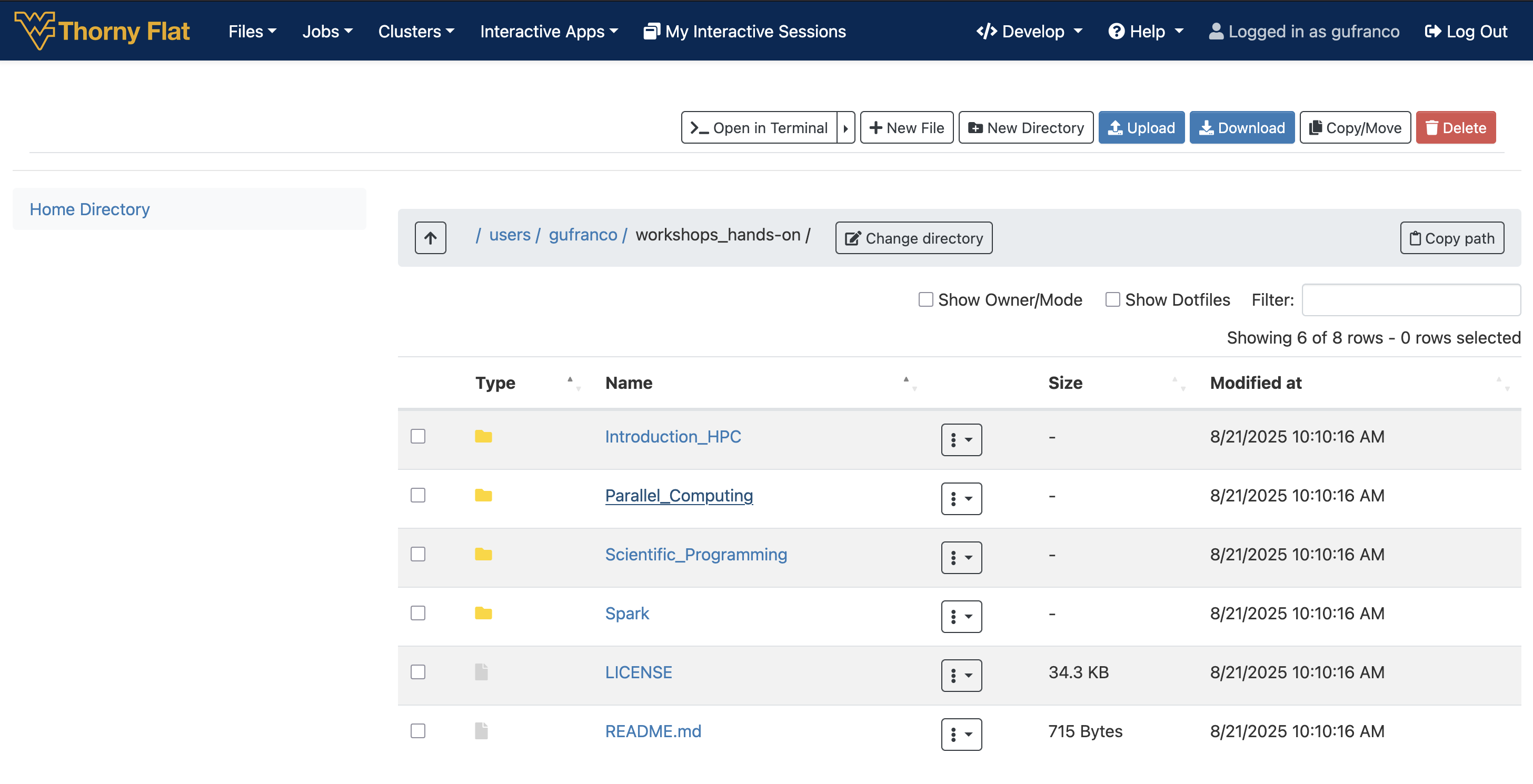
SFT
SFTP (Secure File Transfer Protocol) provides a secure way to transfer files between a local system and a remote server. The commands used within an SFTP session are similar to standard Unix-like shell commands but are specific to managing files and directories on both the local and remote systems.
Research Computing a dedicated server for transferring files to/from Thorny Flat. This is a low level and scriptable interface.
Connecting
Initiates an SFTP connection to the specified remote host using the given username.
~$ sftp <username>@tf-data.hpc.wvu.edu This works very similar to a SSH connection. You need to enter the password followed by the MFA (DUO in 2025). Once your credentials are accepted you land on a prompt like this:
Connected to tf-data.hpc.wvu.edu.
sftp>
From this interface you execute commands that allow you to list the remote files, download and upload files and recursive commands for operating with entire folders.
Navigation and Listing
The SFTP protocol offers commands to interact with the remote and
local filesystems. There are commands like ls,
cd and pwd operating on the remote side and
commands with the prefix l such as lls,
lcd and lpwd that will do the equivalent
operation on the local filesystem.
This is the list of commands for both remote and local operation:
-
ls: Lists files and directories on the remote system. -
lls: Lists files and directories on the local system. -
cd [directory]: Changes the current working directory on the remote system. -
lcd [directory]: Changes the current working directory on the local system. -
pwd: Displays the current working directory on the remote system. -
lpwd: Displays the current working directory on the local system.
File Transfer
SFT provides commands to download (get) or upload files (put) and there are commands for one, several and entire folders.
-
get [remote_file] [local_path]: Downloads a file from the remote system to the local system. -
put [local_file] [remote_path]: Uploads a file from the local system to the remote system. -
mget [remote_files]: Downloads multiple files from the remote system. -
mput [local_files]: Uploads multiple files to the remote system. -
get -R [remote_directory]: Recursively downloads a directory and its contents. -
put -R [local_directory]: Recursively uploads a directory and its contents.
File and Directory Management
Same as on Unix-like shell commands, we have commands for creating folders, both on the remote and local filesystem, remove and rename files and change permissions for files on the remote system.
-
mkdir [directory]: Creates a new directory on the remote system. -
lmkdir [directory]: Creates a new directory on the local system. -
rmdir [directory]: Removes an empty directory on the remote system. -
rm [file]: Deletes a file on the remote system. -
rename [old_path] [new_path]: Renames a file or directory on the remote system. -
chmod [mode] [path]: Changes file permissions on the remote system. -
chown [owner] [path]: Changes the owner of a file on the remote system. -
chgrp [group] [path]: Changes the group of a file on the remote system.
Help and finish session
-
help: Displays a list of available SFTP commands. -
exit,quit, orbye: Terminates the SFTP session.
SFT from a GUI interface
For users who are more comfortable with Graphical User Interfaces, you may want to utilize one of the following clients:
WINSCP WinSCP is a popular SFTP client and FTP client for Microsoft Windows! Copy file between a local computer and remote servers using FTP, FTPS, SCP, SFTP, WebDAV or S3 file transfer protocols.
FILEZILLA FileZilla Client not only supports FTP, but also FTP over TLS (FTPS) and SFTP. It is open source software distributed free of charge under the terms of the GNU General Public License. It support several OSes such as Windows, macOS and Linux.
Globus Online
Globus Online is the preferred method for transferring files to, from, and between HPC clusters. There are several advantages to using Globus compared to other methods that will be covered on File Transfer Section: We can summarize the advantages as:
Globus works from a web browser, not need to learn commands for a terminal.
Transfers are done in the background so users do not need to keep the browser open. The transfer happens behind the curtains.
Auto performance tuning to ensure the data is transferred as quickly as possible. One can expect a speedup of at least 2x over traditional transfer methods.
Transfers can work in parallel, and data could be encrypted during transfer.
The integrity of the transfer can be ensured via checksum methods (Hashes).
Transfers are automatically restarted after a failed or stopped connection.
Ability to only transfer files that have yet to be transferred (similar to rsync).
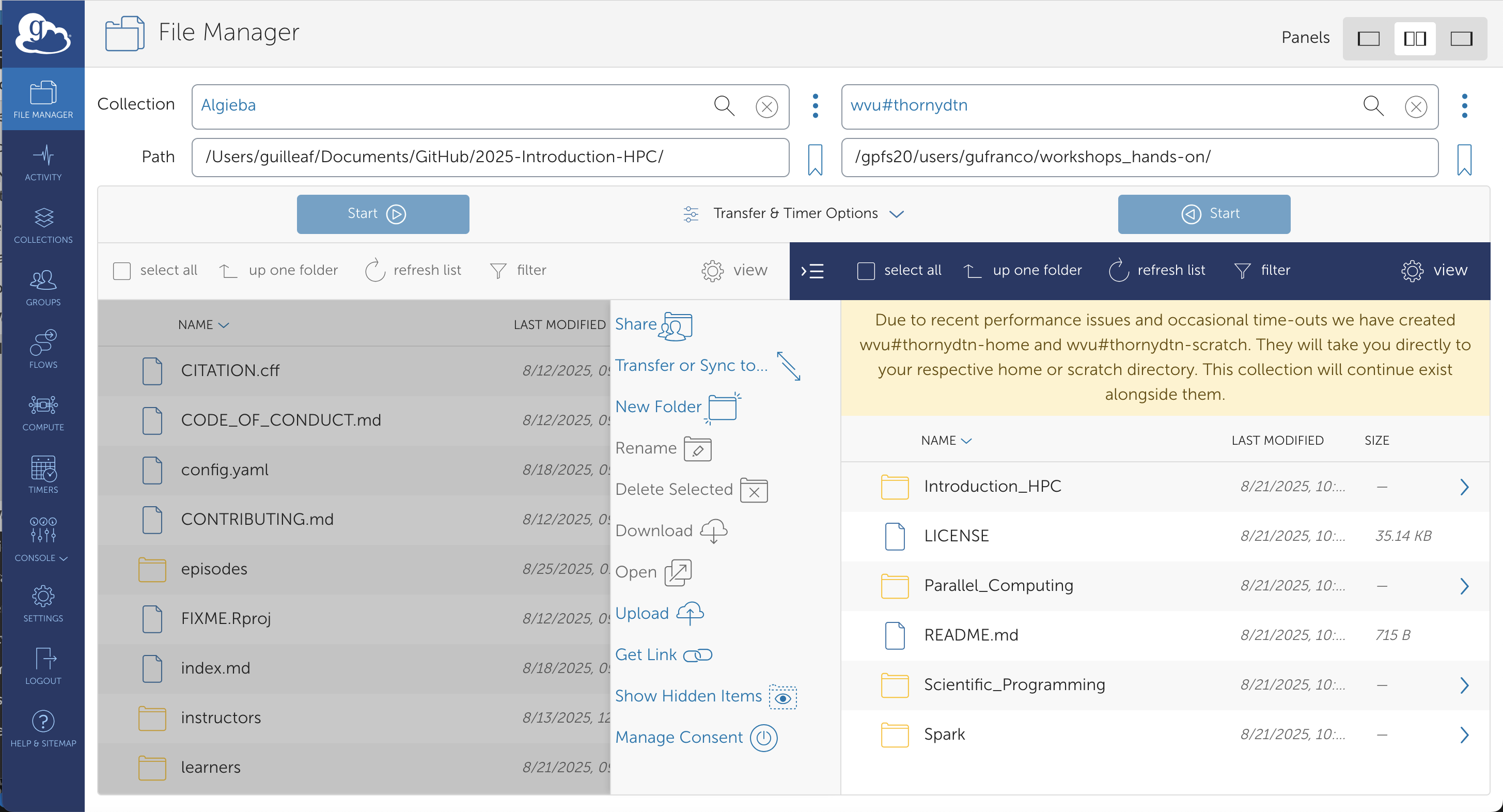
Connecting to the Globus Web App
To be able to move data in and out the HPC cluster to your own computer, there are two tasks to be completed. Link Globus to your personal WVU account so you can access the end points to our clusters and download and install “Globus Connect Personal” which is a small piece of software that will transfor your own computer into an endpoint where you can interchange data with the HPC cluster.
The steps are very simple all from your web browser and after a few minutes you will have setup the end points and will be able to tranfer files. The first step is to connect Globus Homepage.
Once the initial page of globus is displayed, clic on the top right corner over Log in

Once you are authenticated you end on the Globus File Manager. There are several options on your left and three ways of showing panels on the top right.
The next step is to install Globus Connect Personal. The application to convert your own computer into a endpoint. Click on Collections on the left side bar
On the top right corner you will see a link to Get Globus Connect Personal. Click there to go to the Download page for the software.
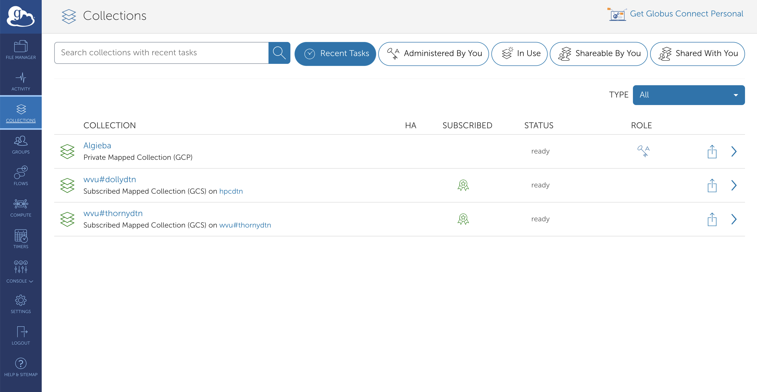
Once you have installed the Globus Connect Personal you are ready to download files from/to your computer to/from the remote machine.
- “Supercomputers are far more powerful than desktop computers”
- “Most supercomputers today are HPC clusters”
- “Supercomputers are intended to run large calculations or simulations that takes days or weeks to complete”
- “HPC clusters are aggregates of machines that operate as a single entity to provide computational power to many users”
Content from Workload Manager: Slurm
Last updated on 2025-08-18 | Edit this page
Overview
Questions
- “What is a resource manager, a scheduler, and a workload manager?”
- “How do we submit a job on an HPC cluster?”
Objectives
- “Submit a job and have it completed successfully.”
- “Understand how to make resource requests.”
- “Submit an interactive job.”
- “Learn the most frequently used SLURM commands”
Introduction
Imagine for a moment that you need to execute a large simulation and all that you have is the computer that is in front of you. You will initiate the simulation by launching the program that will compute it. You ajust the parameters to avoid overloading the machine with more concurrent operations than the machine can process efficiently. It is possible that you cannot do anything else with the computer until the simulation is finished.
Changing the situation a bit, now you have several computers at your disposal and you have many simulations to do, maybe the same simulation but under different physical conditions. You will have to connect to each computer to start the simulation and periodically monitor the computers to check if some of them have finished and its ready to run a new simulation.
Moving to an even more complex scenario. Consider the case of several users, each wanting to run many simulations like yours and having a number of computers capable of runing all those simulations. Coordinating all the work and all the executions could be a daunting task that can be solved if a program could take care or mapping all the jobs from all the users to the available resources and monitoring when one computer can take another job.
All what we have described is the work of two programs, a resource manager in charge of monitoring the state of a pool of computers and a scheduler that will assign jobs to the different machines as fairly as possible for all the users in the cluster. In the case of our cluster those two roles are managed by a single software called Slurm and the integration of the resource manager, scheduler with the addition and accounting and other roles makes Slurm to be called a Workload Manager.
An HPC system such as Thorny Flat or Dolly Sods has tenths nodes and more than 100 users. How do we decide who gets what and when? How do we ensure that a task is run with the resources it needs? This job is handled by a special piece of software called the scheduler. The scheduler manages which jobs run where and when on an HPC system.
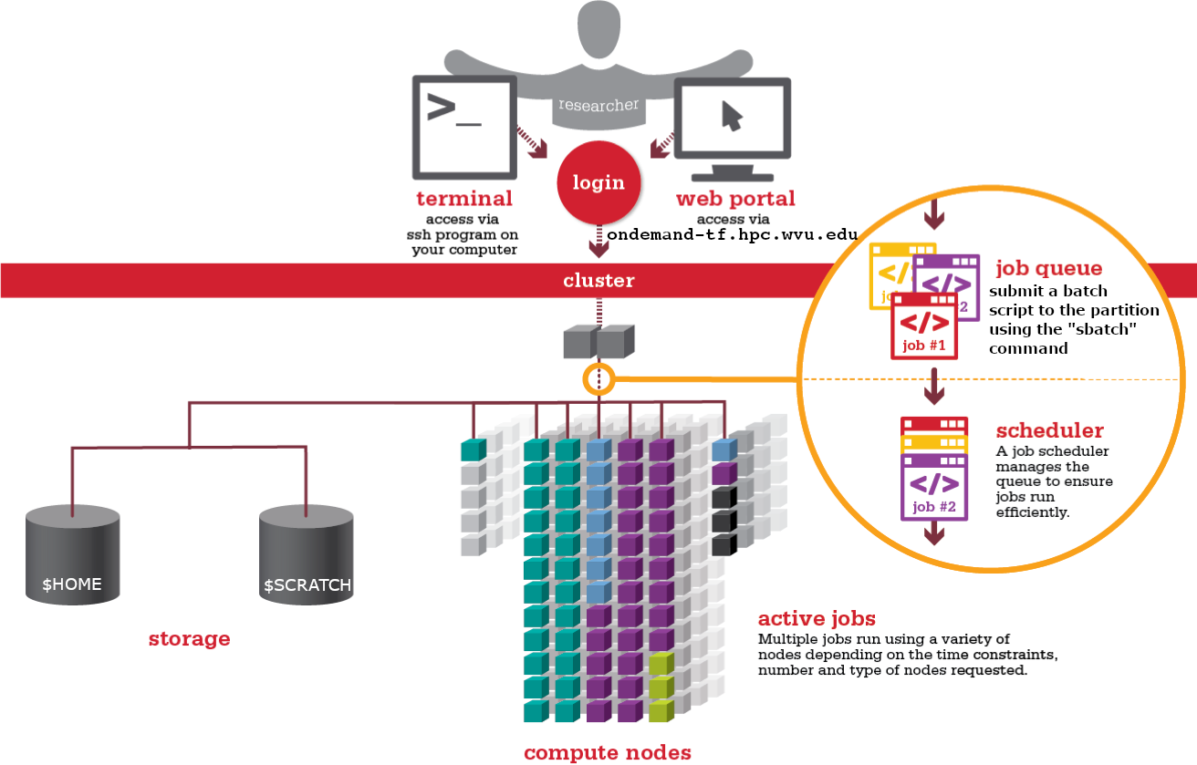
The scheduler used on our clusters is SLURM. SLURM is not the only resource manager or scheduler for HPC systems. Other software packages offer similar functionality. The exact syntax might change, but the concepts remain the same.
A Resource Manager takes care of receiving job submissions and executes those jobs when resources are available, providing the most efficient conditions for the jobs. On the other hand, a job scheduler is in charge of associating jobs with the appropriate resources and trying to maximize an objective function, such as total utilization constrained by priorities and the best balance between the resources requested and resources available. As SLURM is taking the dual role of Resource Manager and Scheduler, SLURM calls itself a Workload Manager, a term that better embraces the multiple roles taken by this software package.
Workload Manager on WVU Clusters
All of our clusters use Slurm as Workload Manager. On Thorny Flat, we
have a compatibility layer so that most Torque/Moab batch scripts will
still work. If you are new to WVU’s HPC clusters, it makes the most
sense to learn the SLURM batch commands.
See Slurm Quick
Start Guide for more SLURM information.
What is a Batch Script?
The most basic use of the scheduler is to run a command non-interactively. This is also referred to as batch job submission. In this case, we need to make a script that incorporates some arguments for SLURM, such as the resources needed and the modules that need to be loaded.
We will use the sleep.sh job script as an example.
Parameters
Let’s discuss the example SLURM script, sleep.sh. Go to
File Explorer and edit sleep.sh
~$ cd $HOME
~$ mkdir SLEEP
~$ cd SLEEP
~$ nano sleep.sh
Write the following in the file with your text editor:
#!/bin/bash

#SBATCH --partition=standby
#SBATCH --job-name=test_job
#SBATCH --time=00:03:00
#SBATCH --nodes=1 --ntasks-per-node=2

echo 'This script is running on:'
hostname
echo 'The date is :'
date
sleep 120
Comments in UNIX (denoted by #) are typically ignored.
But there are exceptions. For instance, the special #!
comment at the beginning of scripts specifies what program should be
used to run it (typically /bin/bash). This is required in
SLURM so don’t leave it out! Schedulers like SLURM also have a special
comment used to denote special scheduler-specific options. Though these
comments differ from scheduler to scheduler, SLURM’s special comment is
#SBATCH. Anything following the #SBATCH
comment is interpreted as an instruction to the scheduler.
In our example, we have set the following parameters:
| Option | Name | Example Setting | Notes |
|---|---|---|---|
--partition |
queue | standby | See next section for queue info |
--job-name |
jobname | test_script | Name of your script (no spaces, alphanumeric only) |
--time |
total job time | multiple settings | See next segment |
--nodes |
nodes requested | multiple settings | See next segment |
--ntasks-per-node |
cores per node | multiple settings | See next segment |
Resource list
A resource list will contain a number of settings that inform the scheduler what resources to allocate for your job and for how long (wall time).
Walltime
Walltime is represented by --time=00:03:00 in the format
HH:MM:SS. This will be how long the job will run before timing out. If
your job exceeds this time, the scheduler will terminate the job. You
should find a usual runtime for the job and add some more (say 20%) to
it. For example, if a job took approximately 10 hours, the wall time
limit could be set to 12 hours, e.g. “–time=12:00:00”. By setting the
wall time, the scheduler can perform job scheduling more efficiently and
also reduces occasions where errors can leave the job stalled but still
taking up resources for the default much longer wall time limit (for
queue wall time defaults, run squeue command)
Walltime test exercise
Resource requests are typically binding. If you exceed them, your job will be killed. Let’s use wall time as an example. We will request 30 seconds of wall time, and attempt to run a job for two minutes.
#!/bin/bash

#SBATCH --partition=standby
#SBATCH --job-name=test_job
#SBATCH --time=00:00:30
#SBATCH --nodes=1 --ntasks-per-node=2

echo 'This script is running on:'
hostname
echo 'The date is :'
date
sleep 120
Submit the job and wait for it to finish. Once it has finished, check the error log file. In the error file, there will be
This script is running on:
This script is running on:
taicm002.hpc.wvu.edu
The date is :
Thu Jul 20 19:25:21 EDT 2023
slurmstepd: error: *** JOB 453582 ON taicm002 CANCELLED AT 2023-07-20T19:26:33 DUE TO TIME LIMIT ***
What happened?
Our job was killed for exceeding the amount of resources it requested. Although this appears harsh, this is a feature. Strict adherence to resource requests allows the scheduler to find the best possible place for your jobs. Even more importantly, it ensures that another user cannot use more resources than they’ve been given. If another user messes up and accidentally attempts to use all of the CPUs or memory on a node, SLURM will either restrain their job to the requested resources or kill the job outright. Other jobs on the node will be unaffected. This means that one user cannot mess up the experience of others, the only jobs affected by a mistake in scheduling will be their own.
Compute Resources and Parameters
Compute parameters The argument --nodes specifies the
number of nodes (or chunks of resource) required;
--ntasks-per-node indicates the number of CPUs per chunk
required.
| nodes | tasks | Description |
|---|---|---|
| 2 | 16 | 32 Processor job, using 2 nodes and 16 processors per node |
| 4 | 8 | 32 Processor job, using 4 nodes and 8 processors per node |
| 8 | 28 | 244 Processor job, using 8 nodes and 28 processor per node |
| 1 | 40 | 40 Processor job, using 1 nodes and 40 processors per node |
Each of these parameters has a default setting they will revert to if not set; however, this means your script may act differently to what you expect.
You can find more information about these parameters by viewing the
manual page for the sbatch function. This will also show
you what the default settings are.
$> man sbatchSetting up email notifications
Jobs on an HPC system might run for days or even weeks. We probably
have better things to do than constantly check on the status of our job
with squeue. Looking at the online documentation for
sbatch (you can also google “sbatch slurm”), can you
set up our test job to send you an email when it finishes?
Hint: you will need to use the --mail-user and
--mail-type options.
Running a batch job (two methods)
Submit Jobs with job composer on OnDemand
OnDemand also has a tool for job creation and submission to the batch system. The same information as above applies since it still uses the same underlying queue system. In the Job Composer, you can create a new location in your home directory for a new job, create or transfer a job script and input files, edit everything, and submit your job all from this screen.
We will run this job in the Job Composer by creating a new job from specified path.
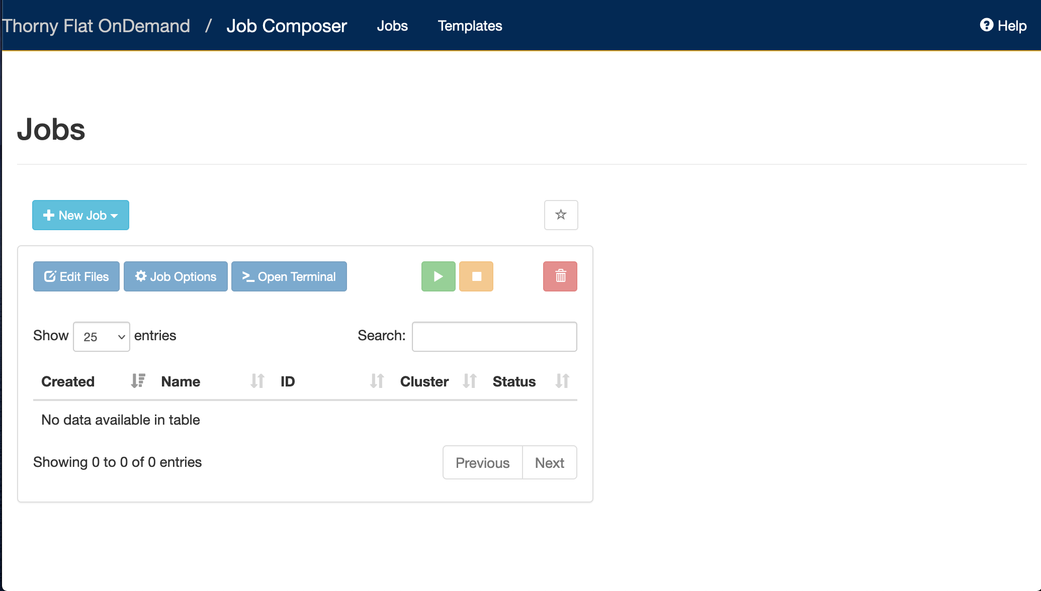
You’ll see the Job Options page, like this:
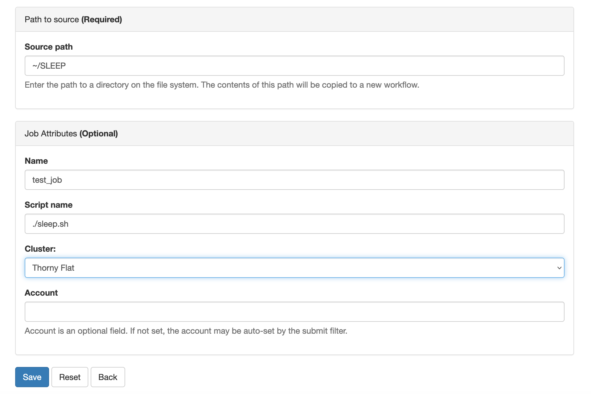
Fill it in as shown. Path is ~/SLEEP and then select
Save.
To run the job, select green ‘play’ button.
If the job is successfully submitted, a green bar will appear on the top of the page.
Also, OnDemand allows you to view the queue for all systems (not just the one you are on in the shell) under Jobs, select Active Jobs. You can filter by your jobs, your group’s jobs, and all jobs.
Submitting Jobs via the command line
To submit this job to the scheduler, we use the sbatch
command.
~$ sbatch sleep.sh
Submitted batch job 453594
~$
The number that first appears is your Job ID. When the job is completed, you will get two files: an Output and an Error file (even if there is no errors). They will be named {JobName}.o{JobID} and {JobName}.e{JobID} respectively.
And that’s all we need to do to submit a job. To check on our job’s
status, we use the command squeue.
~$ squeue -u $USER
             JOBID PARTITION     NAME     USER ST       TIME  NODES NODELIST(REASON)
            453594   standby test_job gufranco  R       0:34      1 taicm009
We can see all the details of our job, most importantly if it is in
the “R” or “RUNNING” state. Sometimes our jobs might need to wait in a
queue (“PD”) or have an error. The best way to check our job’s status is
with squeue. It is easiest to view just your own jobs in
the queue with the squeue -u $USER. Otherwise, you get the
entire queue.
Partitions (Also known as queues)
There are usually a number of available partitions (Other resource managers call them queues) to use on the HPC clusters. Each cluster has separate partitions. The same compute node can be associated with multiple partitions Your job will be routed to the appropriate compute node based on the list of nodes associated with the partition, the wall time, and the computational resources requested. To get the list of partitions on the cluster, execute:
	$> sinfo -s
	PARTITION       AVAIL  TIMELIMIT   NODES(A/I/O/T) NODELIST
	standby*           up    4:00:00      94/71/2/167 taicm[001-009],tarcl100,tarcs[100,200-206,300-304],tbdcx001,tbmcs[001-011,100-103],tbpcm200,tbpcs001,tcbcx100,tcdcx100,tcgcx300,tcocm[100-104],tcocs[001-064,100],tcocx[001-003],tcscm300,tjscl100,tjscm001,tmmcm[100-108],tngcm200,tpmcm[001-006],tsacs001,tsdcl[001-002],tsscl[001-002],ttmcm[100-101],tzecl[100-107],tzecs[100-115]
	comm_small_day     up 1-00:00:00        59/5/1/65 tcocs[001-064,100]
	comm_small_week    up 7-00:00:00        59/5/1/65 tcocs[001-064,100]
	comm_med_day       up 1-00:00:00          5/0/0/5 tcocm[100-104]
	comm_med_week      up 7-00:00:00          5/0/0/5 tcocm[100-104]
	comm_xl_week       up 7-00:00:00          3/0/0/3 tcocx[001-003]
	comm_gpu_inter     up    4:00:00         8/1/2/11 tbegq[200-202],tbmgq[001,100],tcogq[001-006]
	comm_gpu_week      up 7-00:00:00          5/0/1/6 tcogq[001-006]
	aei0001            up   infinite          3/5/1/9 taicm[001-009]
	alromero           up   infinite        12/2/0/14 tarcl100,tarcs[100,200-206,300-304]
	be_gpu             up   infinite          1/1/1/3 tbegq[200-202]
	bvpopp             up   infinite          0/1/0/1 tbpcs001
	cedumitrescu       up   infinite          1/0/0/1 tcdcx100
	cfb0001            up   infinite          0/1/0/1 tcbcx100
	cgriffin           up   infinite          1/0/0/1 tcgcx300
	chemdept           up   infinite          0/4/0/4 tbmcs[100-103]
	chemdept-gpu       up   infinite          1/0/0/1 tbmgq100
	cs00048            up   infinite          0/1/0/1 tcscm300
	jaspeir            up   infinite          0/2/0/2 tjscl100,tjscm001
	jbmertz            up   infinite        3/14/0/17 tbmcs[001-011,100-103],tbmgq[001,100]
	mamclaughlin       up   infinite          1/8/0/9 tmmcm[100-108]
	ngarapat           up   infinite          0/1/0/1 tngcm200
	pmm0026            up   infinite          0/6/0/6 tpmcm[001-006]
	sbs0016            up   infinite          0/2/0/2 tsscl[001-002]
	spdifazio          up   infinite          0/2/0/2 tsdcl[001-002]
	tdmusho            up   infinite          1/5/0/6 taicm[001-004],ttmcm[100-101]
	vyakkerman         up   infinite          1/0/0/1 tsacs001
	zbetienne          up   infinite        6/18/0/24 tzecl[100-107],tzecs[100-115]
	zbetienne_large    up   infinite          6/2/0/8 tzecl[100-107]
zbetienne_small up infinite 0/16/0/16 tzecs[100-115]Exercise: Submitting resource requests
Submit a job that will use 1 node, 4 processors, and 5 minutes of walltime.
Job environment variables
Slurm sets multiple environment variables at submission time. The following variables are commonly used in command files:
| Variable Name | Description |
|---|---|
$SLURM_JOB_ID |
Full jobid assigned to this job. Often used to uniquely name output
files for this job, for example: srun - np 16 ./a.out >output.\({SLURM_JOB_ID}|
|
`\)SLURM_JOB_NAME| Name of the job. This can be set using the --job-name option in the SLURM script (or from the command line). The default job name is the name of the SLURM script.| |\(SLURM_JOB_NUM_NODES` | Number of nodes allocated
|
|
`\)SLURM_JOB_PARTITION| Queue job was submitted to.| |\(SLURM_NTASKS` | The number of processes
requested|
|
`\)SLURM_SUBMIT_DIR| The directory from which the batch job was submitted. | |$SLURM_ARRAY_TASK_ID` |
Canceling a job
Sometimes we’ll make a mistake and need to cancel a job. This can be
done with the qdel command. Let’s submit a job and then
cancel it using its job number.
~$ sbatch sleep.sh
Submitted batch job 453599

$> $ squeue -u $USER
             JOBID PARTITION     NAME     USER ST       TIME  NODES NODELIST(REASON)
            453599   standby test_job gufranco  R       0:47      1 tcocs015
Now cancel the job with it’s job number. Absence of any job info indicates that the job has been successfully canceled.
~$ scancel 453599
~$ squeue -u $USER
             JOBID PARTITION     NAME     USER ST       TIME  NODES NODELIST(REASON)
Detailed information about jobs
The information provided by the command squeue is
sometimes not enough, and you would like to gather a complete picture of
the state of a particular job. The command scontrol
provides a wealth of information about jobs but also partitions and
nodes. Information about a job:
	$ sbatch sleep.sh
	Submitted batch job 453604
	$ scontrol show job 453604
	JobId=453604 JobName=test_job
	   UserId=gufranco(318130) GroupId=its-rc-thorny(1079001) MCS_label=N/A
	   Priority=11588 Nice=0 Account=its-rc-admin QOS=normal
	   JobState=RUNNING Reason=None Dependency=(null)
	   Requeue=0 Restarts=0 BatchFlag=1 Reboot=0 ExitCode=0:0
	   RunTime=00:00:19 TimeLimit=00:04:00 TimeMin=N/A
	   SubmitTime=2023-07-20T20:39:15 EligibleTime=2023-07-20T20:39:15
	   AccrueTime=2023-07-20T20:39:15
	   StartTime=2023-07-20T20:39:15 EndTime=2023-07-20T20:43:15 Deadline=N/A
	   PreemptEligibleTime=2023-07-20T20:39:15 PreemptTime=None
	   SuspendTime=None SecsPreSuspend=0 LastSchedEval=2023-07-20T20:39:15 Scheduler=Main
	   Partition=standby AllocNode:Sid=trcis001:31864
	   ReqNodeList=(null) ExcNodeList=(null)
	   NodeList=taicm007
	   BatchHost=taicm007
	   NumNodes=1 NumCPUs=2 NumTasks=2 CPUs/Task=1 ReqB:S:C:T=0:0:*:*
	   TRES=cpu=2,node=1,billing=2
	   Socks/Node=* NtasksPerN:B:S:C=2:0:*:* CoreSpec=*
	   MinCPUsNode=2 MinMemoryNode=0 MinTmpDiskNode=0
	   Features=(null) DelayBoot=00:00:00
	   OverSubscribe=OK Contiguous=0 Licenses=(null) Network=(null)
	   Command=/gpfs20/users/gufranco/SLEEP/sleep.sh
	   WorkDir=/gpfs20/users/gufranco/SLEEP
	   StdErr=/gpfs20/users/gufranco/SLEEP/slurm-453604.out
	   StdIn=/dev/null
	   StdOut=/gpfs20/users/gufranco/SLEEP/slurm-453604.out
	   Power=
Interactive jobs
Sometimes, you will need a lot of resources for interactive use. Perhaps it’s the first time running an analysis, or we are attempting to debug something that went wrong with a previous job.
You can also request interactive jobs on OnDemand using the Interactive Apps menu.
To submit an interactive job requesting 4 cores on the partition standby and with a wall time of 40 minutes, execute:
~$ srun -p standby -t 40:00 -c 4 --pty bashAnother example includes requesting a GPU compute compute, execute:
~$ srun -p comm_gpu_inter -G 1 -t 2:00:00 -c 8 --pty bash` ## Job arrays
Job arrays offer a mechanism for submitting and managing collections of similar jobs quickly and easily; job arrays with many tasks can be submitted from a single submission script. Job arrays are very useful for testing jobs when one parameter is changed or to execute the same workflow on a set of samples.
For our example, we will create a folder FIBONACCI and a submission
script called fibo.sh
~$ mkdir FIBONACCI
~$ cd FIBONACCI/
~$ nano fibo.sh
Write the content of the submission script as follows:
	#!/bin/bash

	#SBATCH --partition=standby
	#SBATCH --job-name=test_job
	#SBATCH --time=00:03:30
	#SBATCH --nodes=1 --ntasks-per-node=2
	#SBATCH --array 1-10

	# Static input for N
	N=10

	# First Number of the
	# Fibonacci Series
	a=$SLURM_ARRAY_TASK_ID

	# Second Number of the
	# Fibonacci Series
	b=`expr $SLURM_ARRAY_TASK_ID + 1`

	echo "10 first elements in the Fibonacci Sequence."
	echo ""
	echo "Starting with $a and $b"
	echo ""

	for (( i=0; i<N; i++ ))
	do
	    echo -n "$a "
	    fn=$((a + b))
	    a=$b
	    b=$fn
	done
	# End of for loop
	echo ""
	sleep 60
The array index values on job arrays are specified using the
--array or -a option of the
sbatch command. All the jobs in the job array will have the
same variables except for the environment variable
SLURM_ARRAY_TASK_ID , which is set to its array index
value. This variable can redirect the workflow to a different folder or
execute the simulation with different parameters.
Submit the job array:
~$ sbatch fibo.sh
Submitted batch job 453632
~$ squeue -u $USER
             JOBID PARTITION     NAME     USER ST       TIME  NODES NODELIST(REASON)
          453632_1   standby test_job gufranco  R       0:03      1 taicm007
          453632_2   standby test_job gufranco  R       0:03      1 taicm007
          453632_3   standby test_job gufranco  R       0:03      1 taicm007
          453632_4   standby test_job gufranco  R       0:03      1 taicm007
          453632_5   standby test_job gufranco  R       0:03      1 taicm007
          453632_6   standby test_job gufranco  R       0:03      1 taicm007
          453632_7   standby test_job gufranco  R       0:03      1 taicm007
          453632_8   standby test_job gufranco  R       0:03      1 taicm007
          453632_9   standby test_job gufranco  R       0:03      1 taicm007
         453632_10   standby test_job gufranco  R       0:03      1 taicm007
The job submission will create ten jobs When the jobs finish, their
output will be in files slurm-XXX. For example:
``` ~$ cat slurm-453632_7.out 10 first elements in the Fibonacci Sequence
Starting with 7 and 8
7 8 15 23 38 61 99 160 259 419 ~
- “The scheduler handles how compute resources are shared between users.”
- “Everything you do should be run through the scheduler.”
- “A non-interactive job is expressed as a shell script that is submitted to the cluster.”
- “Try to adjust the wall time to around 10-20% more than the expected time the job should need.”
- “It is a good idea to keep aliases to common torque commands for easy execution.”
Content from Software on HPC Clusters: modules, conda and containers
Last updated on 2025-08-28 | Edit this page
Overview
Questions
- “What are the options to enable software packages on an HPC cluster?”
- “What are the differences between environment modules, conda, and apptainer?”
- “What are environment modules and how to use them?”
- “How do I use and create conda environments?”
- “How do I open a shell and execute commands on an Apptainer/Singularity container?”
Objectives
- “Learn about the three main options to enable software on HPC clusters.”
- “Load and unload environment modules”
- “Activate and change conda environments”
- “Get a shell and execute commands inside singularity containers.”
Introduction
Many jobs are being executed on an HPC cluster daily. Jobs use different software packages or different version of the same package. Each area of science uses its own set of software packages. Sometimes, the same software package is used in multiple versions, and those versions must be available on the same HPC cluster. Different from a machine intended for a single user, offering such variety of software is challenging. To solve all this challenge, several options have been implemented on HPC clusters. There are software pacakges installed by the system administrators but also software packages compiled and/or installed by each user. Software directly installed on host or using some degree of isolation from it. There are different options with various levels of isolation from the host system, and some of these options are better suited for particular kinds of software.
Environment Modules
Environment modules are a mechanism that easily enables software by allowing administrators to install non-regular locations and the user to adapt his/her environment to access those locations and use the software installed there. By changing specific variables on the shell, different versions of packages can be made visible to the shell or to a script. Environment modules is a software package that gives the user the ability to change the variables that the shell uses to find executables and libraries. To better understand how environment modules do their job it is essential to understand the concept of variables in the shell and the particular role of special variables called environment variables
Shell variables and environment variables
The shell is a programming language in itself. As with any
programming language, it has the ability to define placeholders for
storing values. Those placeholders are called variables and the shell
commands and shell scripts can be made use of them. Shell variables can
be created on the shell using the operator =. For
example:
~$ A=10
~$ B=20
Environment variables are shell variables that are exported, i.e., converted into global variables. The shell and many other command line programs use a set of variables to control their behavior. Those variables are called environment variables Think about them as placeholders for information stored within the system that passes data to programs launched in the shell.
To create an environment variable, you can first to create a variable
and make it and environment variable using the command
export followed by the name of the variable.
~$ A=10
~$ B=20
~$ export A
~$ export B
This procedure can be simplified with a single line that defines and export the variable. Example:
~$ export A=10
~$ export B=20
Environment Variables control CLI functionality. They declare where to search for executable commands, where to search for libraries, which language display messages to you, how you prompt looks. Beyond the shell itself, environment variables are use by many codes to control their own operation.
You can see all the variables currently defined by executing:
~$ envEnvironment variables are similar to the shell variables that you can create of the shell. Shell variables can be used to store data and manipulated during the life of the shell session. However, only environment variables are visible by child processes created from that shell. To clarify this consider this script:
#!/bin/bash

echo A= $A
echo B= $B
C=$(( $A + $B ))
echo C= $C
Now create two shell variables and execute the script, do the same with environment variables and notice that now the script is able to see the variables.
Some common environment variables commonly use by the shell are:
| Environment Variable | Description |
|---|---|
| $USER | Your username |
| $HOME | The path to your home directory |
| $PS1 | Your prompt |
| $PATH | List of locations to search for executable commands |
| $MANPATH | List of locations to search for manual pages |
| $LD_LIBRARY_PATH | List of locations to search for libraries in runtime |
| $LIBRARY_PATH | List of locations to search for libraries during compilation (actually during linking) |
Those are just a few environment variables of common use. There are many more. Changing them will change where executables are found, which libraries are used and how the system behaves in general. That is why managing the environment variables properly is so important on a machine, and even more on a HPC cluster, a machine that runs many different codes with different versions.
Here is where environment modules enter.
Environment Modules
The modules software package allows you to dynamically modify your user environment by using modulefiles.
Each module file contains the information needed to configure the
shell for an application. After the module’s software package is
initialized, the environment can be modified on a per-module basis using
the module command, which interprets module files. Typically, module
files instruct the module command to alter or set shell environment
variables such as PATH, MANPATH, and others.
The module files can be shared by many users on a system, and users can
have their own collection to supplement or replace the shared module
files.
As a user, you can add and remove module files from the current
environment. The environment changes contained in a module file can also
be summarized through the module show command. You are welcome to change
modules in your .bashrc or .cshrc, but be
aware that some modules print information (to standard error) when
loaded. This should be directed to a file or /dev/null when
loaded in an initialization script.
Basic arguments
The following table lists the most common module command options.
| Command | Description |
|---|---|
| module list | Lists modules currently loaded in a user’s environment. |
| module avail | Lists all available modules on a system. |
| module show | Shows environment changes that will be made by loading a given module. |
| module load | Loads a module. |
| module unload | Unloads a module. |
| module help | Shows help for a module. |
| module swap | Swaps a currently loaded module for an unloaded module. |
Exercise: Using modulefiles
Check the modules that you currently have and clean (purge) your environment from them. Check again and confirm that no module is loaded.
Check which versions of Python, R, and GCC you have from the RHEL itself. Try to get and idea of how old those three components are. For python and R, all that you have to do is enter the corresponding command (
Rorpython). For GCC you need to usegcc --versionand see the date of those programs.Now let’s get a newer version of those three components by loading the corresponding modules. Search for the module for Python 3.10.11, R 4.4.1, and GCC 9.3.0 and load the corresponding modules. To make things easier, you can use check the availability of modules just in the languages section.
~$ module avail lang~$ module purge
~$ module load lang/python/cpython_3.11.3_gcc122 lang/r/4.4.1_gcc122 lang/gcc/12.2.0 - Check again which version of those three components you have now.
Notice that in the case of Python 3, the command python still goes
towards the old Python 2.6.6, as the Python 3.x interpreter is not
backward compatible with Python 2.x the new command is called
python3. Check its version by entering the command.
~$ python3 --version- Clean all of the environment
~$ module purge- Go back and purge all the modules from your environment. We will now
explore why it is essential to use a recent compiler. Try to compile the
code at
workshops_hands-on/Introduction_HPC/5._Environment_Modules/lambda_c++14.cpp. Go to the folder and execute:
~$ g++ lambda_c++14.cppAt this point, you should have received a list of errors, that is because even if the code is C++ it uses elements of the language that were not present at that time on C++ Specification. The code actually uses C++14, and only recent versions of GCC allow for these declarations. Let’s check how many GCC compilers we have available on Thorny Flat.
~$ module avail lang/gccNow, from that list, start loading and trying to compile the code as indicated above. Which versions of GCC allow you to compile the code? Also try the Intel compilers. In the case of the Intel compiler, the command to compile the code is:
~$ icpc lambda_c++14.cppTry with all the Intel compilers. It will fail with some of them. That is because the default standard for the Intel C++ compiler is not C++14. You do not need to declare it explicitly, and for Intel Compiler Suite 2021, but for older versions, the correct command line is:
~$ icpc lambda_c++14.cpp -std=c++14It should be clearer why modules are an important feature of any HPC infrastructure, as it allows you to use several compilers, libraries, and packages in different versions. On a normal computer, you usually have just one.
Conda
Conda is an open-source package management system and environment management system. Conda quickly installs, runs, and updates packages and their dependencies. Conda easily creates, saves, loads, and switches between environments. It was created for Python programs, but it can package and distribute software for any language.
Conda, as a package manager, helps you find and install packages. If you need a package that requires a different version of Python, you do not need to switch to a different environment manager because conda is also an environment manager. With just a few commands, you can set up a totally separate environment to run that different version of Python while continuing to run your usual version of Python in your normal environment.
There are two installers for conda, Anaconda and Miniconda.
Anaconda vs Miniconda
Anaconda is a downloadable, free, open-source, high-performance, and optimized Python and R distribution. Anaconda includes conda, conda-build, Python, and 100+ automatically installed, open-source scientific packages and their dependencies that have been tested to work well together, including SciPy, NumPy, and many others. Ananconda is more suited to be installed on a desktop environment as you get, after installation, a fairly complete environment for scientific computing.
On the other hand, Miniconda is a minimalistic installer for conda. Miniconda is a small, bootstrap version of Anaconda that includes only conda, Python, the packages they depend on, and a small number of other useful packages, including pip, zlib, and a few others. Miniconda is more suited for HPC environments where a minimal installation is all that is needed, and users can create their own environments as needed.
Activating Conda on Thorny Flat and Dolly Sods
On Thorny Flat, the command to activate conda is:
~$ source /shared/software/conda/conda_init.shOr you can see the command line trying to load the module for conda
~$ module load condaAfter activation, you are positioned in the base
environment.
When you have activated conda, you are always inside a
conda environment. Initially, you start on the base
environment, and your prompt in the shell will include a prefix in
parentheses indicating the name of the conda environment you are
currently using.
Conda Environments
Conda allows you to change your environment easily. It also gives you
tools to create new environments, change from one environment to
another, and install packages and their dependencies. Conda environments
will not interact with other environments, so you can easily keep
different versions of packages just by creating multiple
conda environments and populating those with the various
versions of software you want to use.
When you begin using conda, you already have a default environment
named base. You cannot install packages on the
base environment as that is a centrally managed
environment. You can, however, create new environments for installing
packages. Try to keep separate environments for different packages or
groups of packages. That reduces the chances of incompatibility between
them.
Knowing which environments are available
At the time of this tutorial (2024), Thorny Flat offers the following environments centrally installed::
~$ conda env list

(base) trcis001:~$ conda env list
# conda environments:
#
base                    * /shared/software/conda
abienv_py36               /shared/software/conda/envs/abienv_py36
abienv_py37               /shared/software/conda/envs/abienv_py37
cutadaptenv               /shared/software/conda/envs/cutadaptenv
genomics_2024             /shared/software/conda/envs/genomics_2024
materials_2024            /shared/software/conda/envs/materials_2024
materials_2024_gcc93      /shared/software/conda/envs/materials_2024_gcc93
materials_discovery       /shared/software/conda/envs/materials_discovery
moose                     /shared/software/conda/envs/moose
neural_gpu                /shared/software/conda/envs/neural_gpu
picrust                   /shared/software/conda/envs/picrust
picrust2                  /shared/software/conda/envs/picrust2
python27                  /shared/software/conda/envs/python27
python35                  /shared/software/conda/envs/python35
python36                  /shared/software/conda/envs/python36
python37                  /shared/software/conda/envs/python37
qiime2-2022.8             /shared/software/conda/envs/qiime2-2022.8
qiime2-2023.2             /shared/software/conda/envs/qiime2-2023.2
qiime2-amplicon-2023.9    /shared/software/conda/envs/qiime2-amplicon-2023.9
qiime2-shotgun-2023.9     /shared/software/conda/envs/qiime2-shotgun-2023.9
qiime2-tiny-2023.9        /shared/software/conda/envs/qiime2-tiny-2023.9
r_4.2                     /shared/software/conda/envs/r_4.2
scipoptsuite              /shared/software/conda/envs/scipoptsuite
sourcetracker2            /shared/software/conda/envs/sourcetracker2
st2_py36                  /shared/software/conda/envs/st2_py36
st2_py37                  /shared/software/conda/envs/st2_py37
tensorflow18-py36         /shared/software/conda/envs/tensorflow18-py36
Activating an existing environment
Suppose that you want to use the environment called “tpd0001”. To activate this environment, execute::
~$ conda activate tpd0001Deactivating the current environment
The current environment can be deactivated with::
~$ conda deactivateIf you are in the base environment, the deactivation
will not have any effect. You are always at least in the
base environment.
Create a new environment
We will name the environment snowflakes and install the package BioPython. At the Anaconda Prompt or in your terminal window, type the following::
(base) trcis001:~$ conda create --name snowflakes
Retrieving notices: ...working... done
Channels:
 - https://conda.software.inl.gov/public
 - conda-forge
Platform: linux-64
Collecting package metadata (repodata.json): done
Solving environment: done

## Package Plan ##

  environment location: /users/gufranco/.conda/envs/snowflakes


Proceed ([y]/n)? y

Preparing transaction: done
Verifying transaction: done
Executing transaction: done
#
# To activate this environment, use
#
#     $ conda activate snowflakes
#
# To deactivate an active environment, use
#
#     $ conda deactivate
From here you can activate your environment and install the packages of your willing.
(base) trcis001:~$ conda activate snowflakes
(snowflakes) trcis001:~$
or if you want also to install a package you can execute::
conda create --name snowflakes -c bioconda biopythonConda collects metadata about the package and its dependencies and produces an installation plan::
Channels:
 - bioconda
 - https://conda.software.inl.gov/public
 - conda-forge
Platform: linux-64
Collecting package metadata (repodata.json): done
Solving environment: done

## Package Plan ##

  environment location: /users/gufranco/.conda/envs/snowflakes

  added / updated specs:
    - biopython


The following packages will be downloaded:

    package                    |            build
    ---------------------------|-----------------
    biopython-1.70             |      np112py36_1         2.6 MB  bioconda
    ca-certificates-2024.7.4   |       hbcca054_0         151 KB  conda-forge
    ld_impl_linux-64-2.40      |       hf3520f5_7         691 KB  conda-forge
    libgcc-ng-14.1.0           |       h77fa898_0         822 KB  conda-forge
    libgomp-14.1.0             |       h77fa898_0         446 KB  conda-forge
    libpng-1.6.43              |       h2797004_0         281 KB  conda-forge
    libsqlite-3.46.0           |       hde9e2c9_0         845 KB  conda-forge
    libstdcxx-ng-14.1.0        |       hc0a3c3a_0         3.7 MB  conda-forge
    libwebp-base-1.4.0         |       hd590300_0         429 KB  conda-forge
    libzlib-1.2.13             |       h4ab18f5_6          60 KB  conda-forge
    mmtf-python-1.1.3          |     pyhd8ed1ab_0          25 KB  conda-forge
    ncurses-6.5                |       h59595ed_0         867 KB  conda-forge
    numpy-1.12.1               |py36_blas_openblash1522bff_1001         3.8 MB  conda-forge
    reportlab-3.5.68           |   py36h3e18861_0         2.4 MB  conda-forge
    sqlite-3.46.0              |       h6d4b2fc_0         840 KB  conda-forge
    zlib-1.2.13                |       h4ab18f5_6          91 KB  conda-forge
    zstd-1.5.6                 |       ha6fb4c9_0         542 KB  conda-forge
    ------------------------------------------------------------
                                           Total:        18.5 MB

The following NEW packages will be INSTALLED:

  _libgcc_mutex      conda-forge/linux-64::_libgcc_mutex-0.1-conda_forge
  _openmp_mutex      conda-forge/linux-64::_openmp_mutex-4.5-2_gnu
  biopython          bioconda/linux-64::biopython-1.70-np112py36_1
  blas               conda-forge/linux-64::blas-1.1-openblas
  ca-certificates    conda-forge/linux-64::ca-certificates-2024.7.4-hbcca054_0
  freetype           conda-forge/linux-64::freetype-2.12.1-h267a509_2
  jpeg               conda-forge/linux-64::jpeg-9e-h0b41bf4_3
  lcms2              conda-forge/linux-64::lcms2-2.12-hddcbb42_0
  ld_impl_linux-64   conda-forge/linux-64::ld_impl_linux-64-2.40-hf3520f5_7
  lerc               conda-forge/linux-64::lerc-3.0-h9c3ff4c_0
  libdeflate         conda-forge/linux-64::libdeflate-1.10-h7f98852_0
  libffi             conda-forge/linux-64::libffi-3.4.2-h7f98852_5
  libgcc-ng          conda-forge/linux-64::libgcc-ng-14.1.0-h77fa898_0
  libgfortran-ng     conda-forge/linux-64::libgfortran-ng-7.5.0-h14aa051_20
  libgfortran4       conda-forge/linux-64::libgfortran4-7.5.0-h14aa051_20
  libgomp            conda-forge/linux-64::libgomp-14.1.0-h77fa898_0
  libnsl             conda-forge/linux-64::libnsl-2.0.1-hd590300_0
  libpng             conda-forge/linux-64::libpng-1.6.43-h2797004_0
  libsqlite          conda-forge/linux-64::libsqlite-3.46.0-hde9e2c9_0
  libstdcxx-ng       conda-forge/linux-64::libstdcxx-ng-14.1.0-hc0a3c3a_0
  libtiff            conda-forge/linux-64::libtiff-4.3.0-h0fcbabc_4
  libwebp-base       conda-forge/linux-64::libwebp-base-1.4.0-hd590300_0
  libzlib            conda-forge/linux-64::libzlib-1.2.13-h4ab18f5_6
  mmtf-python        conda-forge/noarch::mmtf-python-1.1.3-pyhd8ed1ab_0
  msgpack-python     conda-forge/linux-64::msgpack-python-1.0.2-py36h605e78d_1
  ncurses            conda-forge/linux-64::ncurses-6.5-h59595ed_0
  numpy              conda-forge/linux-64::numpy-1.12.1-py36_blas_openblash1522bff_1001
  olefile            conda-forge/noarch::olefile-0.46-pyh9f0ad1d_1
  openblas           conda-forge/linux-64::openblas-0.3.3-h9ac9557_1001
  openjpeg           conda-forge/linux-64::openjpeg-2.5.0-h7d73246_0
  openssl            conda-forge/linux-64::openssl-1.1.1w-hd590300_0
  pillow             conda-forge/linux-64::pillow-8.3.2-py36h676a545_0
  pip                conda-forge/noarch::pip-21.3.1-pyhd8ed1ab_0
  python             conda-forge/linux-64::python-3.6.15-hb7a2778_0_cpython
  python_abi         conda-forge/linux-64::python_abi-3.6-2_cp36m
  readline           conda-forge/linux-64::readline-8.2-h8228510_1
  reportlab          conda-forge/linux-64::reportlab-3.5.68-py36h3e18861_0
  setuptools         conda-forge/linux-64::setuptools-58.0.4-py36h5fab9bb_2
  sqlite             conda-forge/linux-64::sqlite-3.46.0-h6d4b2fc_0
  tk                 conda-forge/linux-64::tk-8.6.13-noxft_h4845f30_101
  wheel              conda-forge/noarch::wheel-0.37.1-pyhd8ed1ab_0
  xz                 conda-forge/linux-64::xz-5.2.6-h166bdaf_0
  zlib               conda-forge/linux-64::zlib-1.2.13-h4ab18f5_6
  zstd               conda-forge/linux-64::zstd-1.5.6-ha6fb4c9_0


Proceed ([y]/n)?
Conda asks if you want to proceed with the plan::
Proceed ([y]/n)? y
Type "y" and press Enter to proceed.
After that, conda, download, and install the packages, creating a new environment for you. The final message shows how to activate and deactivate the environment::
Preparing transaction: done
Verifying transaction: done
Executing transaction: done
#
# To activate this environment, use
#
#     $ conda activate snowflakes
#
# To deactivate an active environment, use
#
#     $ conda deactivate
Each environment is isolated from other conda environments, and that allows you to keep several environments with different packages on them or different versions of the same packages. As the message shows, you activate the environment with::
~$ conda activate snowflakesNotice that when you activate a new environment, the prompt changes, adding a prefix in parenthesis to indicate which conda environment you are using at that moment. To check the environments available, execute::
~$ conda env listor
~$ conda info --envsConda and Python
When you create a new environment, conda installs the same Python version used to install conda on Thorny Flat (3.9). If you want to use a different version of Python, for example, Python 2.7, create a new environment and specify the version of Python that you want::
~$ conda create --name python27 python=2.7You activate the environment::
~$ conda activate python27And verify the Python version::
~$ python --version
Python 2.7.16 :: Anaconda, Inc.
Conda has packages for versions of python for 2.7, 3.5, 3.6 and 3.7
Managing packages and channels
New packages can be installed to existing conda environments. First search for packages with::
~$ conda search mklPackages are stored in repositories called channels.
By default, conda search on the pkgs/main channel only.
However, there are many other packages on several other channels.
The most prominent channels to search for packages are intel, conda-forge and bioconda To search for packages there execute::
~$ conda search -c intel mkl

~$ conda search -c conda-forge nitime

~$ conda search -c bioconda blast
Packages can be installed on the current environment with::
~$ conda install -c conda-forge nitimeIn this case conda will pick the most recent version of the package compatible with the packages already present on the current environment. You can also be very selective on version and build that you want for the package. First get the list of versions and builds for the package that you want::
~$ conda search -c intel mkl
  Loading channels: done
  # Name                       Version           Build  Channel
  mkl                         2017.0.3         intel_6  intel
  mkl                         2017.0.4      h4c4d0af_0  pkgs/main
  mkl                         2018.0.0      hb491cac_4  pkgs/main
  mkl                         2018.0.0         intel_4  intel
  mkl                         2018.0.1      h19d6760_4  pkgs/main
  mkl                         2018.0.1         intel_4  intel
  mkl                         2018.0.2               1  pkgs/main
  mkl                         2018.0.2         intel_1  intel
  mkl                         2018.0.3               1  pkgs/main
  mkl                         2018.0.3         intel_1  intel
  mkl                           2019.0             117  pkgs/main
  mkl                           2019.0             118  pkgs/main
  mkl                           2019.0       intel_117  intel
  mkl                           2019.1             144  pkgs/main
  mkl                           2019.1       intel_144  intel
  mkl                           2019.2       intel_187  intel
  mkl                           2019.3             199  pkgs/main
  mkl                           2019.3       intel_199  intel
  mkl                           2019.4             243  pkgs/main
  mkl                           2019.4       intel_243  intel
  mkl                           2019.5       intel_281  intel
Now, install the package declaring the version and build::
~$ conda install -c intel mkl=2019.4=intel_243
Collecting package metadata (current_repodata.json): done
Solving environment: done

## Package Plan ##

  environment location: /users/gufranco/.conda/envs/test

  added / updated specs:
    - mkl==2019.4=intel_243


The following packages will be downloaded:

    package                    |            build
    ---------------------------|-----------------
    intel-openmp-2019.5        |        intel_281         888 KB  intel
    mkl-2019.4                 |        intel_243       204.1 MB  intel
    tbb-2019.8                 |        intel_281         874 KB  intel
    ------------------------------------------------------------
                                           Total:       205.8 MB

The following NEW packages will be INSTALLED:

  intel-openmp       intel/linux-64::intel-openmp-2019.5-intel_281
  mkl                intel/linux-64::mkl-2019.4-intel_243
  tbb                intel/linux-64::tbb-2019.8-intel_281


Proceed ([y]/n)?


Downloading and Extracting Packages
tbb-2019.8           | 874 KB    | #################################################################################################################################### | 100%
mkl-2019.4           | 204.1 MB  | #################################################################################################################################### | 100%
intel-openmp-2019.5  | 888 KB    | #################################################################################################################################### | 100%
Preparing transaction: done
Verifying transaction: done
Executing transaction: done
Creating a new environment from a YML file
You can create your own environment, one easy way of doing that is via a YML file that describes the channels and packages that you want on your environment. The YML file will look like this, for a simple case when you want one env for bowtie2 (bowtie2.yml)
    name: thorny-bowtie2
    channels:
      - bioconda
      - conda-forge
      - defaults
    dependencies:
      - bowtie2
Another example is this YML file for installing a curated set of basic genomics codes that requires just a few dependencies. (biocore.yml)
name: biocode
channels:
  - bioconda
  - conda-forge
  - defaults
dependencies:
  - bamtools
  - bcftools
  - bedtools
  - hmmer
  - muscle
  - raxml
  - samtools
  - sga
  - soapdenovo-trans
  - soapdenovo2
  - sra-tools
  - vcftools
  - velvet
To create an environment from those YML files you can select one location on your scratch folder
conda env create -p $SCRATCH/bowtie2 -f bowtie2.ymlor for the biocore.yml
conda env create -p $SCRATCH/biocore -f biocore.ymlBy default, new environments are created inside your
$HOME folder on $HOME/.conda
Listing the packages inside one environment
Bowtie2 has a number of dependencies (19 dependencies for 1 package) Notice that only bowtie2 comes from bioconda channel. All other packages are part of conda-forge, a lower level channel.
~$ conda activate $SCRATCH/bowtie2
~$ conda list
# packages in environment at /scratch/gufranco/bowtie2:
#
# Name                    Version                   Build  Channel
bowtie2                   2.3.4.2          py36h2d50403_0    bioconda
bzip2                     1.0.6                h470a237_2    conda-forge
ca-certificates           2018.8.24            ha4d7672_0    conda-forge
certifi                   2018.8.24                py36_1    conda-forge
libffi                    3.2.1                hfc679d8_5    conda-forge
libgcc-ng                 7.2.0                hdf63c60_3    conda-forge
libstdcxx-ng              7.2.0                hdf63c60_3    conda-forge
ncurses                   6.1                  hfc679d8_1    conda-forge
openssl                   1.0.2p               h470a237_0    conda-forge
perl                      5.26.2               h470a237_0    conda-forge
pip                       18.0                     py36_1    conda-forge
python                    3.6.6                h5001a0f_0    conda-forge
readline                  7.0                  haf1bffa_1    conda-forge
setuptools                40.2.0                   py36_0    conda-forge
sqlite                    3.24.0               h2f33b56_1    conda-forge
tk                        8.6.8                         0    conda-forge
wheel                     0.31.1                   py36_1    conda-forge
xz                        5.2.4                h470a237_1    conda-forge
zlib                      1.2.11               h470a237_3    conda-forge
Using a conda environment in a submission script
To execute software in a non-interactive job you need to source the main script, activate the environment that contains the software you need, execute the the scientific code and deactivate the environment. This is a simple example showing that for bowtie2
Deleting an environment
You can execute this command to remove an environment you own.
~$ conda remove --all -p $SCRATCH/bowtie2or
~$ conda env remove -n bowtie2If the environment is named.
More documentation
Conda Documentation <https://conda.io/docs/index.html>__
[https://conda.io/docs/user-guide/tasks/manage-environments.html\ # Managing environments]
Using Bioconda — Bioconda documentation <https://bioconda.github.io/>__
Available packages — Bioconda documentation <https://bioconda.github.io/conda-recipe_index.html>__
Downloading Miniconda
You do not need to install Miniconda on Thorny Flat or Dolly Sods. However, nothing prevents you from having your version of it if you want. Miniconda can be downloaded from::
wget https://repo.continuum.io/miniconda/Miniconda3-latest-Linux-x86_64.sh
sh Miniconda3-latest-Linux-x86_64.shSingularity Containers
Containers are a software technology that allows us to keep control of the environment where a given code runs. Consider for example that you want to run a code in such a way the same code runs on several machines or clusters, ensuring that the same libraries are loaded and the same general environment is present. Different clusters could come installed with different compilers, different Linux distributions and different libraries in general. Containers can be used to package entire scientific workflows, software and libraries, and even data and move them to several compute infrastructures with complete reproducibility.
Containers are similar to Virtual Machines, however, the differences are enough to consider them different technologies and those differences are very important for HPC. Virtual Machines take up a lot of system resources. Each Virtual Machine (VM) runs not just a full copy of an operating system, but a virtual copy of all the hardware that the operating system needs to run. This quickly adds up to a lot of precious RAM and CPU cycles, valuable resources for HPC.
In contrast, all that a container requires is enough of an operating system, supporting programs and libraries, and system resources to run a specific program. From the user perspective, a container is in most cases a single file that contains the file system, ie a rather complete Unix filesystem tree with all libraries, executables, and data that are needed for a given workflow or scientific computation.
There are several container solutions, the most popular probably is Docker, however, the main issue with using docker on HPC is security, despite the name, containers do not actually contain the powers of the user who executes code on them. That is why you do not see Docker installed on an HPC cluster. Using dockers requires superuser access something that on shared resources like an HPC cluster is not typically possible.
Singularity offers an alternative solution to Docker, users can run the prepared images that we are offering on our clusters or bring their own.
For more information about Singularity and complete documentation see: https://singularity.lbl.gov/quickstart
How to use a singularity Image
There are basically two scenarios, interactive execution and job submission.
Interactive Job
If you are using Visit or RStudio, programs that uses the X11 forwarding, ensure to connect first to the cluster with X11 forwarding, before asking for an interactive job. In order to connect into Thorny with X11 forwarding use:
~$ ssh -X <username>@ssh.wvu.edu~$ ssh -X <username>@tf.hpc.wvu.eduOnce you have login into the cluster, create an interactive job with the following command line, in this case we are using standby as queue but any other queue is valid.
~$ salloc -c 4 -p standbyOnce you get inside a compute node, load the module:
~$ module load singularityAfter loading the module the command singularity is available for usage, and you can get a shell inside the image with:
~$ singularity shell /shared/containers/<Image Name>Job Submission
In this case you do not need to export X11, just login into Thorny Flat
~$ ssh <username>@ssh.wvu.edu

ssh <username>@tf.hpc.wvu.edu
Once you have login into the cluster, create a submission script (“runjob.pbs” for this example), in this case we are using standby as queue but any other queue is valid.
BASH
#!/bin/sh

#SBATCH -J SINGULARITY_JOB
#SBATCH -N 1
#SBATCH -c 4
#SBATCH -p standby
#SBATCH -t 4:00:00

module load singularity

singularity exec /shared/containers/<Image Name> <command_or_script_to_run>
Submit your job with
sbatch runjob.pbsExercise 1: Using singularity on the cluster (Interactive)
This exercise propose the use of singularity to access RStudio-server version 2023.12.1-402 and R 4.4.1
Follow the instructions for accessing an interactive session
The image is located at:
/shared/containers/RStudio-server-2023.12.1-402_R-4.4.1_jammy.sif Be sure that you can execute basic R commands. You can get an error message like:
OUTPUT
WARNING: You are configured to use the CRAN mirror at https://cran.rstudio.com/. This mirror supports secure (HTTPS) downloads however your system is unable to communicate securely with the server (possibly due to out of date certificate files on your system). Falling back to using insecure URL for this mirror.That is normal and due to the fact that compute nodes have no Internet access.
Exercise 2: Using singularity on the cluster (Non-interactive)
Create a script that reads a CSV with official statistics of population for US. The file can be downloaded from:
~$ wget https://www2.census.gov/programs-surveys/popest/datasets/2010-2018/state/detail/SCPRC-EST2018-18+POP-RES.csvHowever, the file is also present in the repository for hands-ons
~$ git clone https://github.com/WVUHPC/workshops_hands-on.gitThe folder is
workshops_hands-on/Introduction_HPC/11._Software_Containers_Singularity.
If you are not familiar with R programming, the script is there too.
Notice that you cannot write your script to download the CSV file
directly from the Census Bureau as the compute nodes have no Internet
access. Write a submission script and submit.
Advanced topics
Modules: Creating a private repository
The basic procedure is to locate modules on a folder accessible by
relevant users and add the variable MODULEPATH to your
.bashrc
MODULEPATH controls the path that the module command
searches when looking for modulefiles. Typically, it is set to a default
value by the bootstrap procedure. MODULEPATH can be set
using ’module use’ or by the module initialization script to search
group or personal modulefile directories before or after the master
modulefile directory.
Singularity: Creating your own images
You can create your own Singularity images and use them on our clusters. The only constrain is that images can only be created on your own machine as you need root access to create them.
The procedure that we will show will be executed on a remote machine provided by JetStream, it should the same if you have your own Linux machine and you have superuser access to it.
The creation of images is an interactive procedure. You learn how to put pieces together and little by little you build your own recipe for your image.
Lets start with a very clean image with centos.
The minimal recipe will bring an image from Docker with the latest
version of CentOS. Lets call the file centos.bst
BASH
# Singularity container with centos
#
# This is the Bootstrap file to recreate the image.
#

Bootstrap: docker
From: centos:latest

%runscript
exec echo "The runscript is the containers default runtime command!"

%files

%environment

%labels
AUTHOR username@mail.wvu.edu

%post
echo "The post section is where you can install, and configure your container."
mkdir -p /data/bin
mkdir -p /gpfs
mkdir -p /users
mkdir -p /group
mkdir -p /scratch
touch /usr/bin/nvidia-smi
A few folders are created that help us to link special folders like
/users, /scratch to the host file system.
Other than that the image contains a very small but usable Linux CentOS
machine.
We start with a writable sandboxed version, the exact command varies from machine to machine, but assuming that you can do sudo and the command singularity is available for root execute this:
~$ sudo singularity build --sandbox centos centos.bstUsing container recipe deffile: centos.bst
Sanitizing environment
Adding base Singularity environment to container
Docker image path: index.docker.io/library/centos:latest
Cache folder set to /root/.singularity/docker
Exploding layer: sha256:8ba884070f611d31cb2c42eddb691319dc9facf5e0ec67672fcfa135181ab3df.tar.gz
Exploding layer: sha256:306a59f4aef08d54a38e1747ff77fc446103a3ee3aea83676db59d6d625b02a1.tar.gz
User defined %runscript found! Taking priority.
Adding files to container
Adding environment to container
Running post scriptlet
+ echo 'The post section is where you can install, and configure your container.'
The post section is where you can install, and configure your container.
+ mkdir -p /data/bin
+ mkdir -p /gpfs
+ mkdir -p /users
+ mkdir -p /group
+ mkdir -p /scratch
+ touch /usr/bin/nvidia-smi
Adding deffile section labels to container
Adding runscript
Finalizing Singularity container
Calculating final size for metadata...
Skipping checks
Singularity container built: centos
Cleaning up...The result will be a folder called centos. We can enter
into that folder to learn what we need to install the packages for our
image.
~$ sudo singularity shell --writable centosFor our exercise lets imagine that we want to use a package that opens a window. In particular, we now that we need a package that is called libgraph to get access to the graphics capabilities. The software is not provided by CentOS itself, so we need to compile it. We need to download, compile and install this package. We learn first how to do it and add that learning to the Bootstrap recipe file.
We need:
Download https://www.mirrorservice.org/sites/download.savannah.gnu.org/releases/libgraph/libgraph-1.0.2.tar.gz, so we need
wgetfor that. This is one package that we need to install from yum.We need compilers, and make. So we have to install
gcc,gcc-c++andmakeThe next time to try, you notice that you will also need some extra packages provided by EPEL, devel packages from CentOS and EPEL repositories. The packages are
SDL-develepel-releaseSDL_image-develcompat-guile18-develandguile-devel.
Trial and error move you from the original recipe to this one
(centos-libgraph.bst):
BASH
# Singularity container with centos
#
# This is the Bootstrap file to recreate the image.
#

Bootstrap: docker
From: centos:latest

%runscript
exec echo "The runscript is the containers default runtime command!"

%files

%environment

%labels
AUTHOR username@mail.wvu.edu

%post
echo "The post section is where you can install, and configure your container."

yum -y install wget make gcc gcc-c++ SDL-devel epel-release
yum -y update && yum -y install SDL_image-devel compat-guile18-devel guile-devel

mkdir -p /data/bin
mkdir -p /gpfs
mkdir -p /users
mkdir -p /group
mkdir -p /scratch
touch /usr/bin/nvidia-smi

cd /data
wget https://www.mirrorservice.org/sites/download.savannah.gnu.org/releases/libgraph/libgraph-1.0.2.tar.gz
tar -zxvf libgraph-1.0.2.tar.gz
cd libgraph-1.0.2 && ./configure --prefix=/data && make && make install
Notice that we have added a few lines using yum to
install some packages, we add EPEL on the first line and we use it to
install some extra packages on the second line.
yum -y install wget make gcc gcc-c++ SDL-devel epel-release
yum -y update && yum -y install SDL_image-devel compat-guile18-devel guile-devel
Finally, we use wget to get the sources and build
libgraph. In order to save space on the VM, lets delete the
old folder and create a new one with the new recipe.
sudo rm -rf centos
sudo singularity build --sandbox centos centos-libgraph.bst
The command takes longer and at the end you get libgraph installed at
/data The final step will be use that to test that we are
able to use libgraph with our application. The application is a couple
of very small codes that use libgraph as dependency.
To achieve this we need.
Modify the environment variables
PATHandLD_LIBRARY_PATHto point to the locations where libgraph and our binaries will be located.Copy the sources
circles.candjulia.cto the image and compile it.
The final version of the Bootstrap recipe looks like this
centos-final.bst
BASH
# Singularity container with centos
#
# This is the Bootstrap file to recreate the image.
#

Bootstrap: docker
From: centos:latest

%runscript
exec echo "The runscript is the containers default runtime command!"

%files
julia.c
circles.c
sample.c

%environment
SHELL=/bin/bash
export SHELL
PATH=/data/bin:$PATH
export PATH
LD_LIBRARY_PATH=$LD_LIBRARY_PATH:/data/lib
export LD_LIBRARY_PATH

%labels
AUTHOR username@mail.wvu.edu

%post
echo "The post section is where you can install, and configure your container."
yum -y install wget make gcc gcc-c++ SDL-devel epel-release
yum -y update && yum -y install SDL_image-devel compat-guile18-devel guile-devel
mkdir -p /data/bin
mkdir -p /gpfs
mkdir -p /users
mkdir -p /group
mkdir -p /scratch
touch /usr/bin/nvidia-smi

mv /circles.c /julia.c /sample.c /data

cd /data
wget https://www.mirrorservice.org/sites/download.savannah.gnu.org/releases/libgraph/libgraph-1.0.2.tar.gz
tar -zxvf libgraph-1.0.2.tar.gz
cd libgraph-1.0.2 && ./configure --prefix=/data && make && make install

cd /data
gcc julia.c -o bin/julia -I/data/include -L/data/lib -lgraph -lm
gcc circles.c -o bin/circles -I/data/include -L/data/lib -lgraph -lm
gcc sample.c -o bin/sample -I/data/include -L/data/lib -lgraph -lm
We add a few sample files sample.c,
circles.c and julia.c that uses the old
graphics.h provided by libgraph.
The binaries are sample, cicles and
julia and they are accessible on the command line.
When you have crafted a good recipe with the codes and data that you
need. The last step is to create a final image. The command for that is
below, remembering of deleting the centos folder to save
space.
~$ sudo rm -rf centos
~$ sudo singularity build centos-final.simg centos-final.bst
This is the final image. It is not too big, it contains the packages that we installed from yum, the sources and binaries for libgraph and the sources for the couple of example sources that uses libgraph. The image can be move to any machine with singularity and should be able to run the codes.
Remember that to see the windows you should have and Xserver running on your machine and X11 forwarding on your ssh client.
- Modules. Use
module availto know all the modules on the cluster. - Modules. Use
module load <module_name>to load a module. - Conda. Use
conda env listto list the available environments. - Conda. Use
conda activateto activate a conda environment. - Singularity. Use
singularity shell <container>to get a shell inside the container. - Singularity. Use
singularity exec <container> <command>to execute a command or script inside the container.
Content from Terminal Multiplexing: tmux
Last updated on 2025-08-18 | Edit this page
Overview
Questions
- “What is a Terminal Multiplexer?”
- “How I can become more productive with a terminal multiplexer?”
- “How can I use tmux?”
Objectives
- “Learn to use a terminal multiplexer like tmux”
- “Learn the basic tmux concepts: sessions, windows and panes”
- “Learn how to create new sessions and attach to existing ones”
- “Learn to span new windows and panes and navegate between them”
From terminal emulation to terminal multiplexing
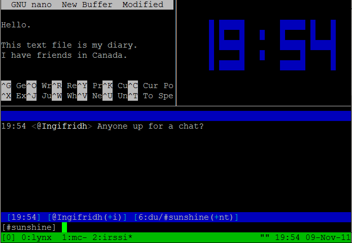
During your interaction with an HPC cluster, you spend most of your time in front of a terminal. You have been working on a terminal during the previous episodes. Let’s now understand more in detail what a terminal is before exploring the concept of terminal multiplexing and tmux in particular.
What you have being using so far to interact with the HPC cluster is called a terminal emulator. In the old days of mainframes (late 70s and 80s), people using computers worked on what were called “dumb terminals”, monitors with a keyboard attached. All real processing happened on a remote machine, the mainframe. Computers at that time were very expensive so at most you were given a keyboard to enter commands and a CRT monitor to see the result of those commands. Many other people could also be using other terminals connected to the same mainframe.
Today, what you have on your hands is a perfectly capable computer, thousands of times more powerful that the mainframes from the 80s. However, there are situations where you need more computational power and for that reason you use a supercomputer such as an HPC cluster. To access these HPC cluster you are using a terminal emulator and an SSH client to connect to a remote machine; the HPC cluster login node.
If you are using a Windows machine, you maybe are using an application such as PuTTy https://www.chiark.greenend.org.uk/~sgtatham/putty/ that will offer a terminal emulator and SSH client on the same package. Despide of ther line being difussed with PuTTY the terminal emulator and SSH client are two different applications. In other Operating Systems like Linux and MacOS the difference between the terminal emulator and the SSH client is more clear.
Now, on your computer, connect to one of our HPC clusters using SSH. You notice that your prompt, the string that indicates that it is ready to receive commands, shows the name of the head node on our clusters. In previous episodes we have learn to execute commands from the terminal, edit text files and submitting jobs.
Imagine that you are editing a text file using any of the three editors from our previous episode. If, for some reason, the internet connection fails, your local computer gets out of power, your SSH session will be closed and the program that you were using to edit the file will closed too. If the editor does not have any recurrent saving mechanism you lost all that you edited and you need to start all over again.
Even if your text editor has some recurring saving mechanism, some work could have been lost, you need to connect to the cluster again, change to the correct working directory before you can continue your work were you were left.
Another limitation of traditional terminals is that you have just one place to enter commands. Working with HPC clusters usually involves working with several jobs and projects, and you would like to edit some text files here, submit new jobs there, check the status of those jobs that you have already submitted, and read the output from the jobs that have been finished. You could open more SSH sessions, but the chances of those sessions failing due to network issues and managing those extra windows limit your ability to work effectively on the cluster.
The solution for the two problems above is using a terminal multiplexer, a program that runs on the login node of the cluster and can continue to work if by change you lost connectivity and gets detached from your local terminal session. tmux is such a terminal multiplexer that it can create multiple emulated terminals.
In this episode we will show you how to create tmux sessions on the cluster and see the effect of detaching and reattaching to the session. Next, we will see the four basic concepts in tmux: Clients, Sessions, Windows and Panes. We will see how to create and move between them and, finally, a few tricks on how to personalize your experience on tmux. As you progress on the use of the cluster tmux will become an important companion for your interaction with the HPC clusters.
tmux lets you switch easily between several virtual
terminals organized in sessions, windows, and panes. One big advantage
of terminal multiplexing is that all those virtual terminals remain
alive when you log out of the system. You can work remotely for a while,
close the connection and reconnect, attach your tmux
session, and continue exactly where you left your work.
Opening a tmux Session and Client
The first concepts in tmux are client and session. A tmux session is made of at least one window that holds at least one pane. We will see about windows and panes later in this episode but right now, lets see how to work with tmux sessions.
First, connect to the cluster using your terminal emulator and SSH client. Once you are connected to the head node of the cluster, execute:
~$ tmuxIf, for some reason, you lost the connection to the server or you detached from the multiplexer, all that you have to do to reconnect is to execute the command:
~$ tmux aYou will see something new here: a green bar on the bottom of your screen. That is the indication that you are inside a tmux session. The tmux status line at the bottom of the screen shows information on the current session. At this point, you have created one tmux client that is attached to the session that was also created. Clients and Sessions are separate entities, allowing you to detach your client from the session and reattach it later. You can also have several clients attached to the same session, and whatever you do on one will be visible on the others. At first sessions and client could be confused, but this exercise will help you understand the concepts.
You are now on a tmux session. Open nano so you can see the top bar and the two command bars on the bottom from the nano session. Write a line like you were writing a text file. All commands inside a session use a prefix key combination. The prefix combination is Ctrl+B, also referred as C-b. You have to press the Ctrl key, keep it pressed and press the B key followed for any command for tmux to interpret. The first command will detach a session from the client. Use the combination C-b d to detach the current session from the client. You will hit the Ctrl key, keep it pressed, and press B, raise both keys, and press D. You will see that the nano top and bottom bars disappear, the green tmux bottom bar also disappears, and you return to your normal terminal. You can go even further and close your terminal on your computer to simulate a loss in internet connection. Reconnect again to the cluster using SSH to return to the head node.
From the head node, we will reattach the session using:
~$ tmux aYou will see your session recovering exactly the same as you left when you detached, and nano should be there with the line that you wrote. You have created your first tmux session and that session will persist until you kill the session or the head node is rebooted, something that happens rarely, usually one or two times per year. For the most part, you can keep your tmux session open
You can create several tmux sessions, each one with a given name, using:
~$ tmux new -s <session_name>Having several sessions is useful if you want a distinctive collection of windows for different projects, as they are more isolated than windows on the same session. Changing between sessions is done with C-b ( and C-b ) to move between the previous and next session. Another way of moving between sessions is using C-b w as we will see next, showing all the windows across all sessions and allowing you to jump into windows from different sessions.
Sessions have names, and those names can be changed with C-b $
Windows and Panes
The next concepts on tmux are windows and panes. A tmux window is the area that fills the entire space offered by your local terminal emulator. Windows has the same purpose as tabs on a browser. When you create your first tmux session, you also create a single window. tmux windows can be further divided in what tmux calls panes. You can divide a single tmux window in multiple panes and you can have several tmux windows on a single tmux session. As we will see in a moment, you can have several tmux sessions attached to tmux clients or detached from them. Each session can hold several tmux windows and each window will have one or more tmux panes. On each of those panes, you will have a shell waiting for your commands. At the end tmux is the equivalent of a window manager in the world of terminals, with the ability to attach and detach at will and running commands concurrently.
In case you are not already attached to the tmux session, enter into the tmux session with:
~$ tmux aYou have one window with one pane inside that fills the entire space. You can create new tmux windows with C-b c. Start creating a few of them. Each new window will appear in the bottom tmux bar. The first ten are identified with a number from a digit number from 0 to 9.
Moving between windows is done using the number associated on the
bottom bar of tmux, to move to the first window (with number 0)
use C-b 0, similarly for all the first 10 windows. You
can create more windows beyond the first 10, but only for those you can
jump into them using the C-b
Notice that windows receive names shown on the bottom bar in tmux. You can change the name of the window using C-b ,. This is useful for generating windows with consistent names for tasks or projects related to the window. You can also use the different windows connected to different machines so the label could be useful to identify which machine you are connected to at a given window.
You can kill the current window with C-b & and see all the windows across all sessions with C-b w. This is another way of moving between windows in different sessions.
The last division in the hierarchy is panes. Panes create new terminals by dividing the window horizontally or vertically. You can create new panes using C-b % for vertical division or C-b “ for horizontal division.
You can move between panes with C-b o or use the
arrows to go to the panes in the direction of the arrow, such as
C-b
One easy way of organizing the panes is using the predefined layouts, and C-b SPACE will cycle between them. Panes can be swapped with C-b { and C-b }. You can zoom into the current pane to take the whole window using C-b z and execute the same command to return to the previous layout.
Copy mode
All the commands above are related to the movement and creation of sessions, windows, and panes. Inside a pane, you can enter Copy mode if you want to scroll the lines on the pane or copy and paste lines. The procedure to use copy mode is as follows:
Press C-b [ to enter in copy mode.
Move the start/end of text to highlight.
Press C-SPACEBAR to start selection. Start highlighting text. Selected text changes the color and background, so you’ll know if the command worked.
Move to the opposite end of the text to copy.
Press ALT-w to copy selected text into tmux clipboard.
Move cursor to opposite tmux pane, or completely different tmux window. Put the cursor where you want to paste the text you just copied.
Press C-b ] to paste copied text from tmux clipboard.
If you work from a Mac, the ALT key (In macOS called option) will not work. One alternative is to use vi-copy mode:
Press C-b : and write: setw -g mode-keys vi
Now enter in copy mode with C-b [
To start selecting the text, use SPACEBAR
Move to the opposite end of the text to copy
Copy the selection with ENTER
Go to the window and pane you want to paste
Press C-b ] to paste copied text from tmux clipboard.
Final remarks
tmux is far more than the few commands shown here. There are many ways to personalize the environment. Some personalizations involve editing the file $HOME/.tmux.conf
Consider for example, this .tmux.conf that changes several colors in the tmux status bar.
######################
### DESIGN CHANGES ###
######################

# loud or quiet?
set -g visual-activity off
set -g visual-bell off
set -g visual-silence off
setw -g monitor-activity off
set -g bell-action none

#  modes
setw -g clock-mode-colour colour5
setw -g mode-style 'fg=colour1 bg=colour18 bold'

# panes
set -g pane-border-style 'fg=colour19 bg=colour0'
set -g pane-active-border-style 'bg=colour0 fg=colour9'

# statusbar
set -g status-position bottom
set -g status-justify left
set -g status-style 'bg=colour18 fg=colour137 dim'
set -g status-left ''
set -g status-right '#[fg=colour233,bg=colour19] %d/%m #[fg=colour233,bg=colour8] %H:%M:%S '
set -g status-right-length 50
set -g status-left-length 20

setw -g window-status-current-style 'fg=colour1 bg=colour19 bold'
setw -g window-status-current-format ' #I#[fg=colour249]:#[fg=colour255]#W#[fg=colour249]#F '

setw -g window-status-style 'fg=colour9 bg=colour18'
setw -g window-status-format ' #I#[fg=colour237]:#[fg=colour250]#W#[fg=colour244]#F '

setw -g window-status-bell-style 'fg=colour255 bg=colour1 bold'

# messages
set -g message-style 'fg=colour232 bg=colour16 bold'
There are a lot of things that can be changed to everyone’s taste.
There are several .tmux.conf files shared on GitHub and
other repositories that customize tmux in several ways.
Exercise: tmux Sessions, Windows and Panes
This exercise will help you familiarize yourself with the three concepts in TMUX.
Create three sessions on TMUX, and give each of them different names, either creating the session with the name or using C-b $ to rename session names.
In one of those sessions, create two windows, and in the other, create three windows. Move between sessions to accomplish this.
In one of those windows, split the window vertically, on another horizontally, and on the third one create 3 panes and cycle between the different layouts using C-b SPACE
Detach or close your terminal and reconnect, attach your sessions, and verify that your windows and panes remain the same.
Exercise: Using tmux
Using the tables above, follow this simple challenge with tmux
Log in to Thorny Flat and create a
tmuxsessionInside the session, create a new window
Go back to window 0 and create a horizontal pane, and inside one of those panes, create a vertical pane.
Create a big clock pane
Detach from your current session, close your terminal, and reconnect. Log in again on Thorny Flat and reattach your session.
Now that you are again in your original session create a new session. You will be automatically redirected there. Leave your session and check the list of sessions.
Kill the second session (session ID is 1)
Reference of tmux commands
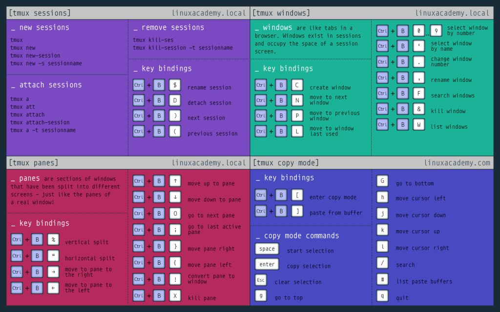
In tmux, by default, the prefix is Ctrl+b. Use the prefix followed by one of the options below:
Windows (tabs)
    c  create window
    w  list windows
    n  next window
    p  previous window
    f  find window
    ,  name window
    &  kill window
Panes (splits)
    %  vertical split
    "  horizontal split
    o  swap panes
    q  show pane numbers
    x  kill pane
    +  break pane into window (e.g. to select text by mouse to copy)
    -  restore pane from window
    ⍽  space - toggle between layouts
    q (Show pane numbers, when the numbers show up type the key to goto that pane)
    { (Move the current pane left)
    } (Move the current pane right)
    z toggle pane zoom
Copy model
[ Copy modeIn copy mode, use these commands to copy a region to the tmux clipboard.
    Ctrl SPACE  Start Selection
    Alt w       Copy the selection to the clipboard
After this use the command to paste
] Paste from clipboardCommand line arguments for tmux
    tmux ls                       list sessions
    tmux new                      new session
    tmux rename -t <ID> new_name  rename a session
tmux kill-session -t <ID> kill session by target- “A terminal multiplexer protects programs such as text editors that are running on the login node from connection drops”
- “Allow programs running on a remote server to be accessed from multiple different local computers.”
- “Work with multiple programs and shells together in one terminal, a bit like a window manager.”